Project 1
CS180/280A: Intro to Computer Vision and Computational Photography
Images of the Russian Empire: Colorizing the Prokudin-Gorskii photo collection

Approach (High-Level)
Goal: Reconstruct a clean color image by extracting the three monochrome plates (B, G, R), aligning them precisely, and stacking them into an RGB image with minimal artifacts.
I first inspected the input plates. There is clear correlation across channels at the same pixel locations: brighter pixels in one channel are usually brighter in the others (not always, but mostly). However, overall illumination and contrast differ between channels, so raw intensities are on different scales.
This suggested using a pixelwise distance metric to quantify alignment quality: if the plates are well aligned, the sum of per-pixel distances should be small. To avoid getting stuck in local minima (which can happen if you only move greedily in the locally best direction), I evaluate the total distance for many candidate shifts and choose the shift with the lowest global score.
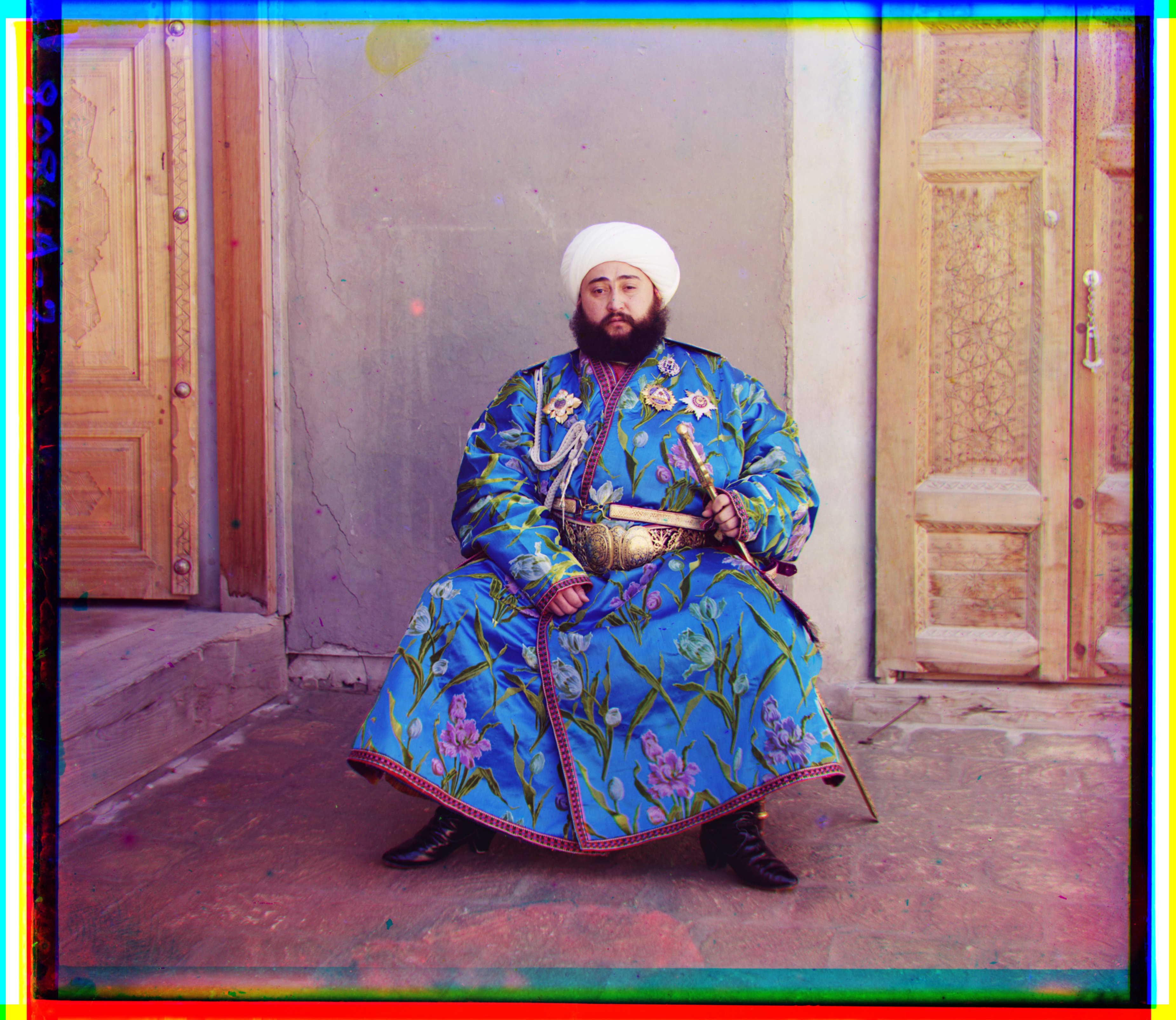
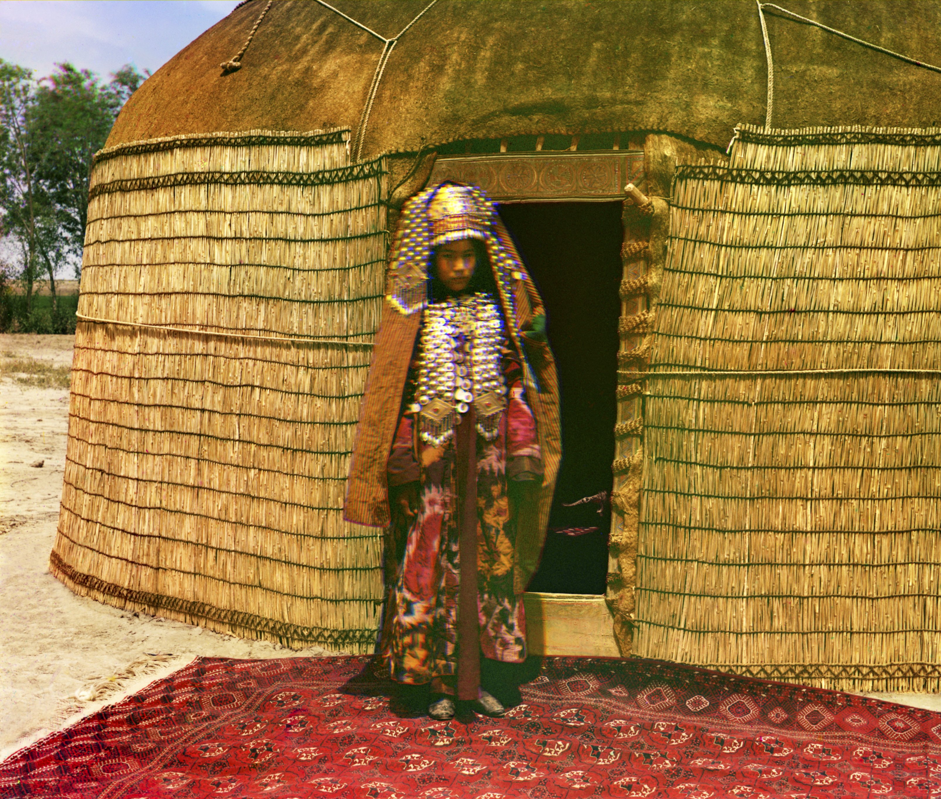
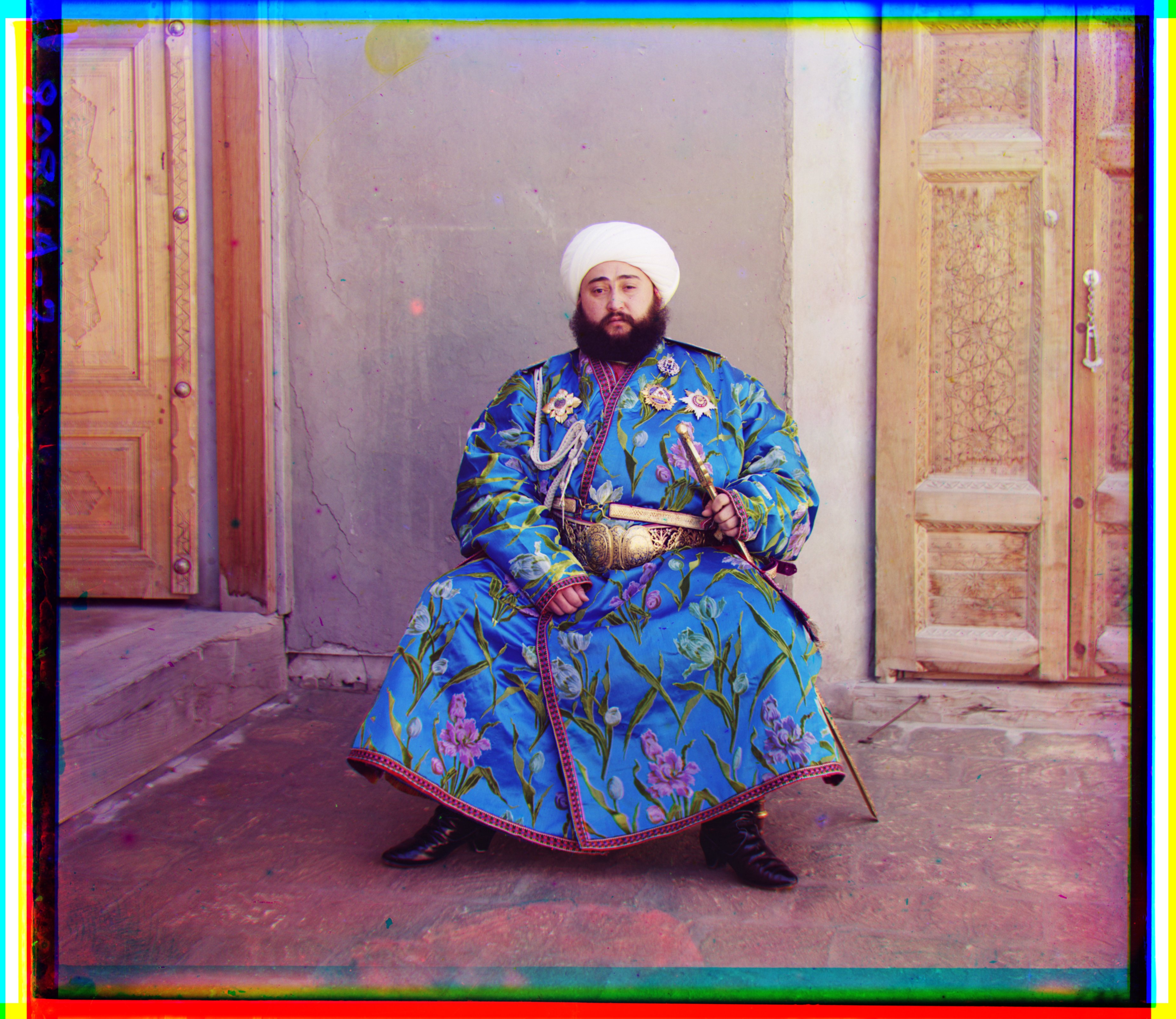
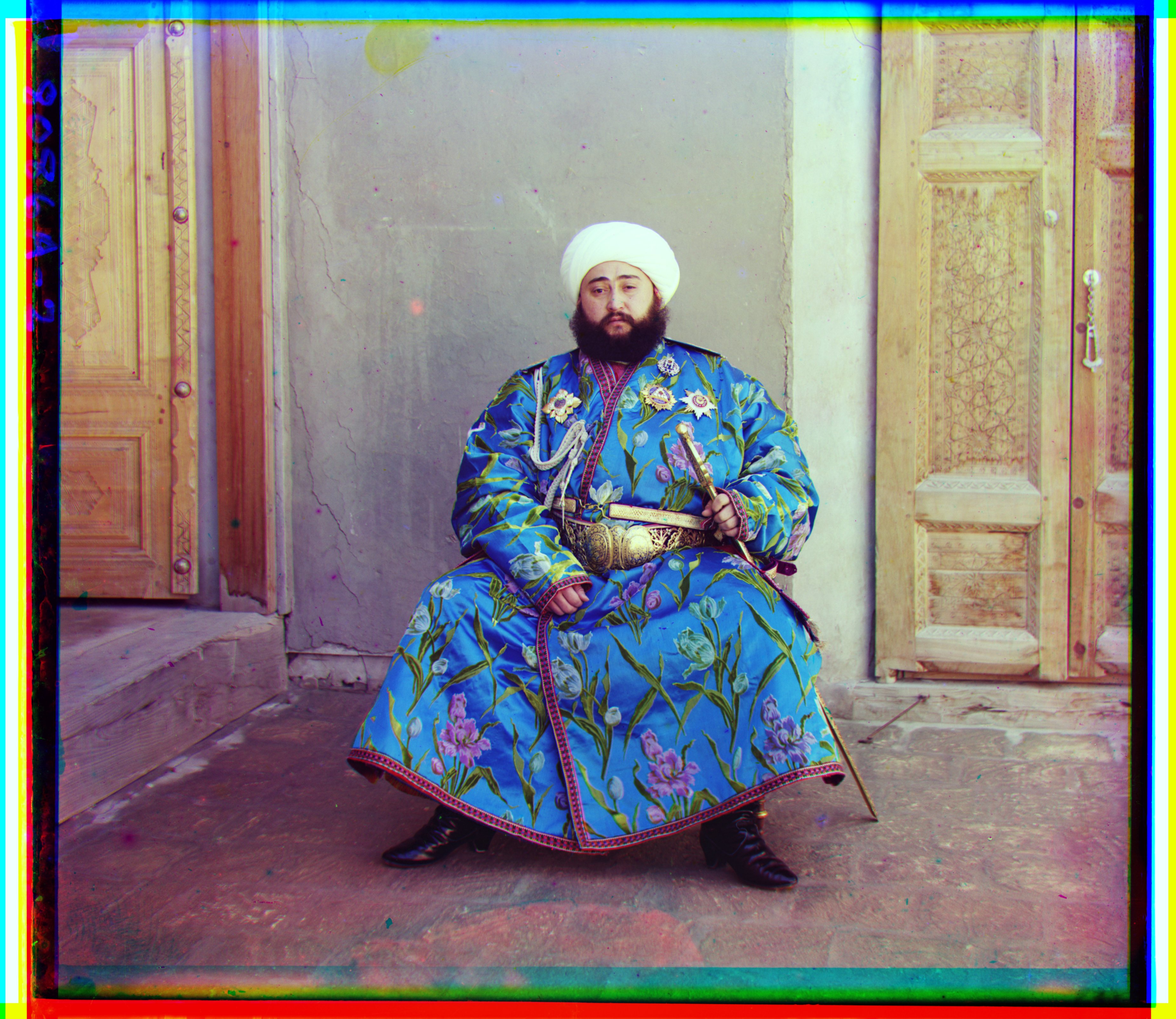
I started with an exhaustive search over translations using the L2 distance on raw pixel values. This already produced good alignments for many images. However, some cases like the emir still failed due to cross‑channel brightness differences, for example clearly visible in his very colorful dress.
I first tried per‑channel min–max scaling to normalize dynamic range, but results were unstable since extrema are image‑dependent and sensitive to outliers. I then switched to per‑channel z‑normalization (standardizing to zero mean and unit variance) before scoring so that structures became more comparable across channels despite overall brightness/gain differences.
L2 distance between two patches/channels I and J:
Z-normalization of a channel X:
Despite z‑normalization, a few images remained challenging. I therefore added Normalized Cross‑Correlation (NCC) as the matching score. Intuition: NCC compares zero‑mean, normalized patches and is invariant to linear brightness/contrast changes, making it better suited when channels have different gains.
In practice, I z‑normalize or zero‑center patches and evaluate NCC over a search window derived by splitting each channel into a small grid of patches; I score candidate shifts across these windows and take the displacement with the highest overall score. This made the alignment robust across all images, including difficult cases like the emir.
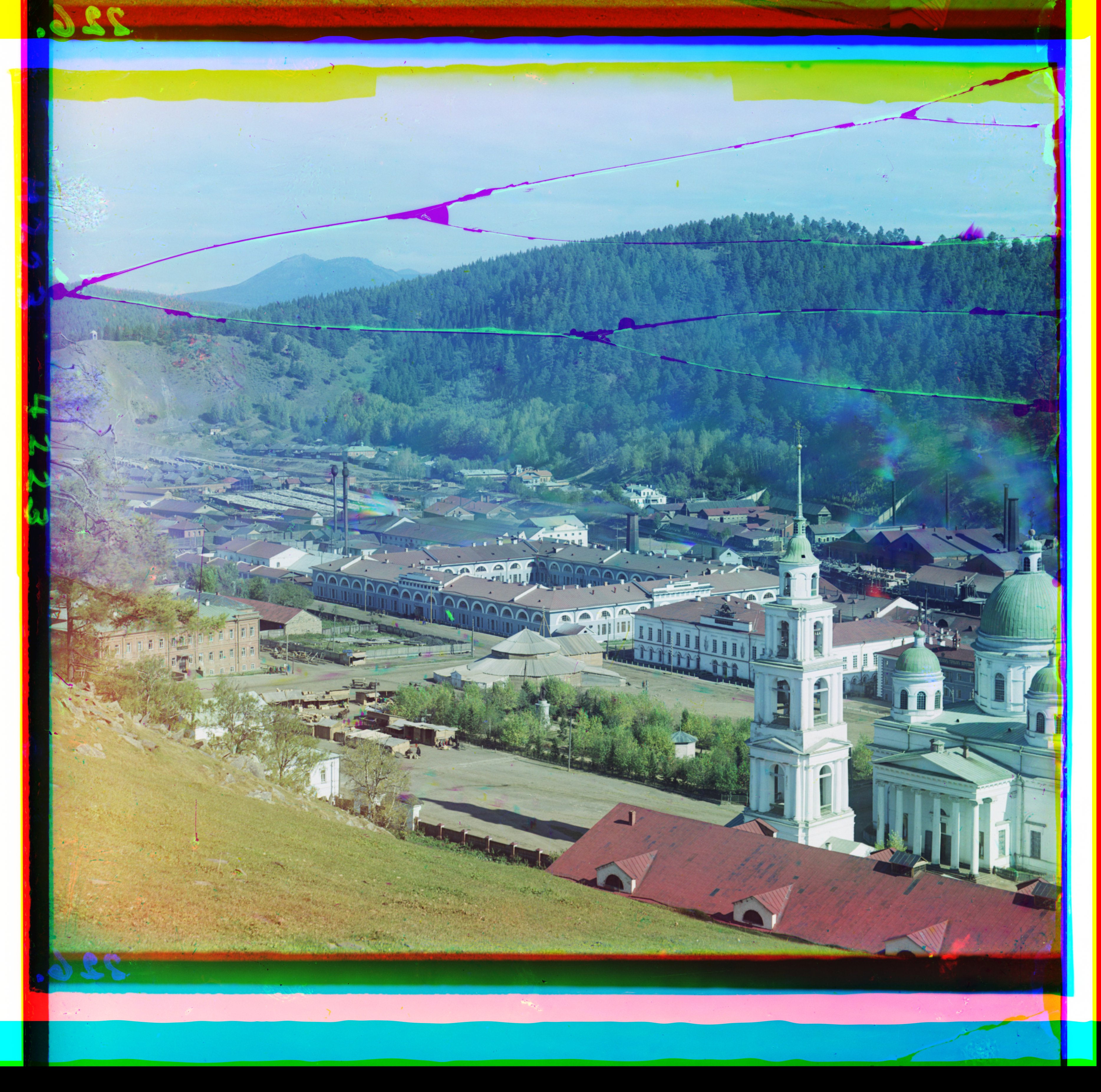
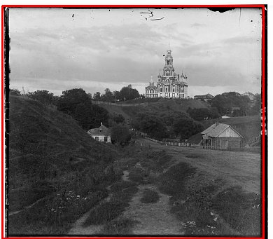
Low‑resolution results (JPEG, brute force)
However, because high‑resolution TIFFs are also available, a faster approach is needed for those larger images.
Coarse‑to‑Fine Pyramid
To make alignment efficient on large glass plates, I use a multi-scale (coarse‑to‑fine) image pyramid:
Intuition: Computing scores (e.g., L2, NCC) over many shifts on full‑resolution images is expensive. Start at a much smaller resolution to get a cheap, rough alignment; then iteratively double the size and refine around that estimate. This minimizes the total number of evaluations overall, with only a few refinements needed at full resolution.
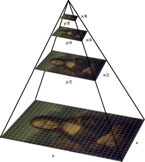
Source: IIPImage documentation
- Build a pyramid by halving resolution until another downscale would make the smallest dimension < 32 px (min base ≈ 32×32).
- At the coarsest level, stack the channels and run an exhaustive search with a ±8 px radius to find the best translation.
- Propagate the displacement to the next finer level (scale ×2), then refine within a small local window of ±2 px (top/bottom/left/right).
- Repeat to full resolution, optionally re‑normalizing and scoring on interior pixels to avoid border effects.
NCC windowing: at the smallest level I split the image into a 2×2 grid and evaluated NCC per cell; at the next level (2× bigger) into a 4×4 grid, and so on. This keeps the NCC window size approximately constant in absolute terms across scales.
Using a larger window (±8) only at the coarsest level and a tighter window (±2) at finer levels dramatically reduces the global search space while preserving final alignment accuracy.
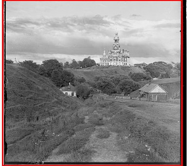
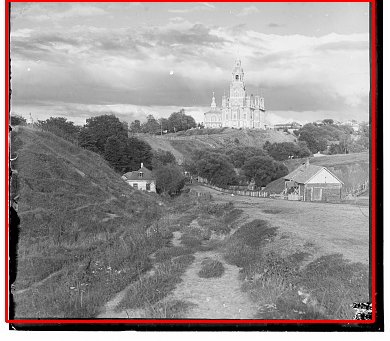
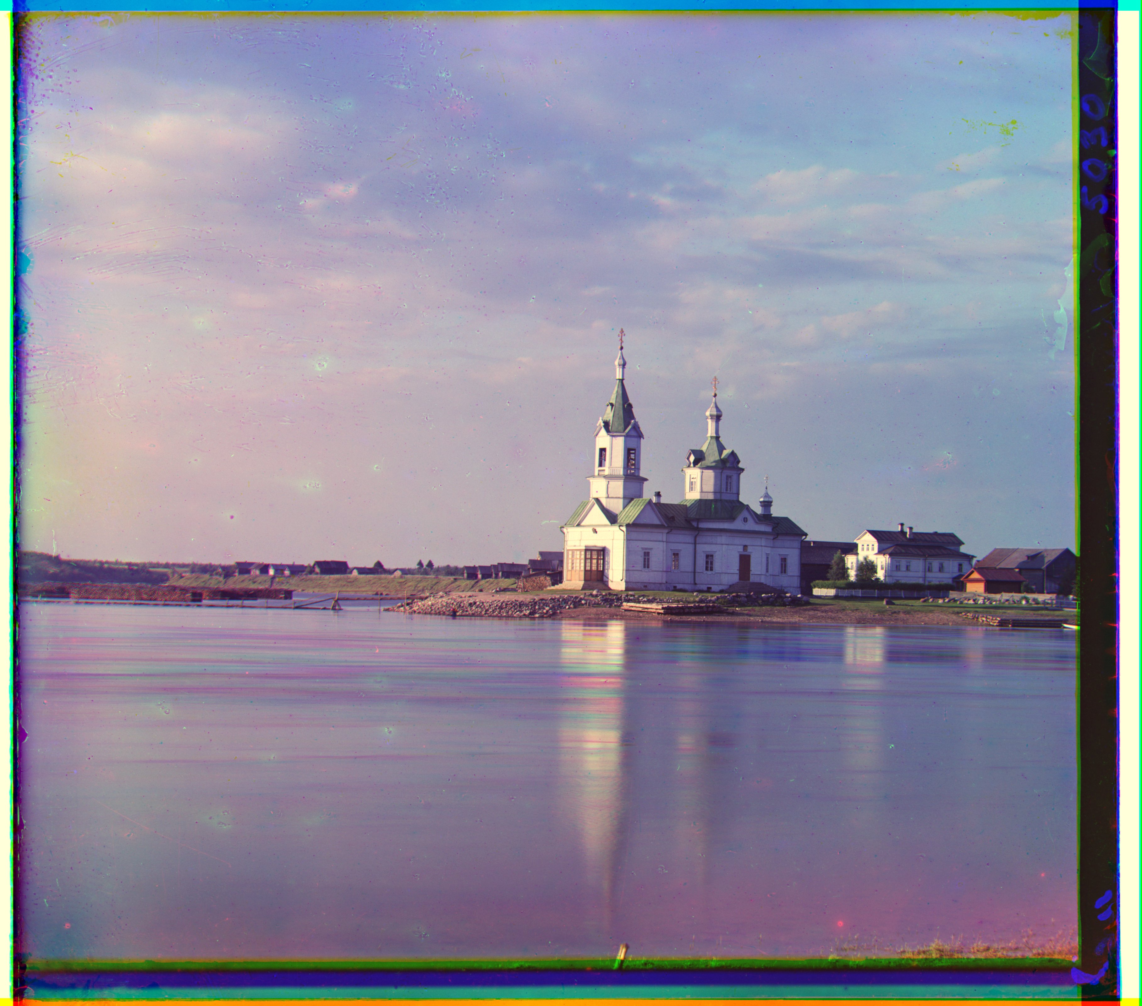
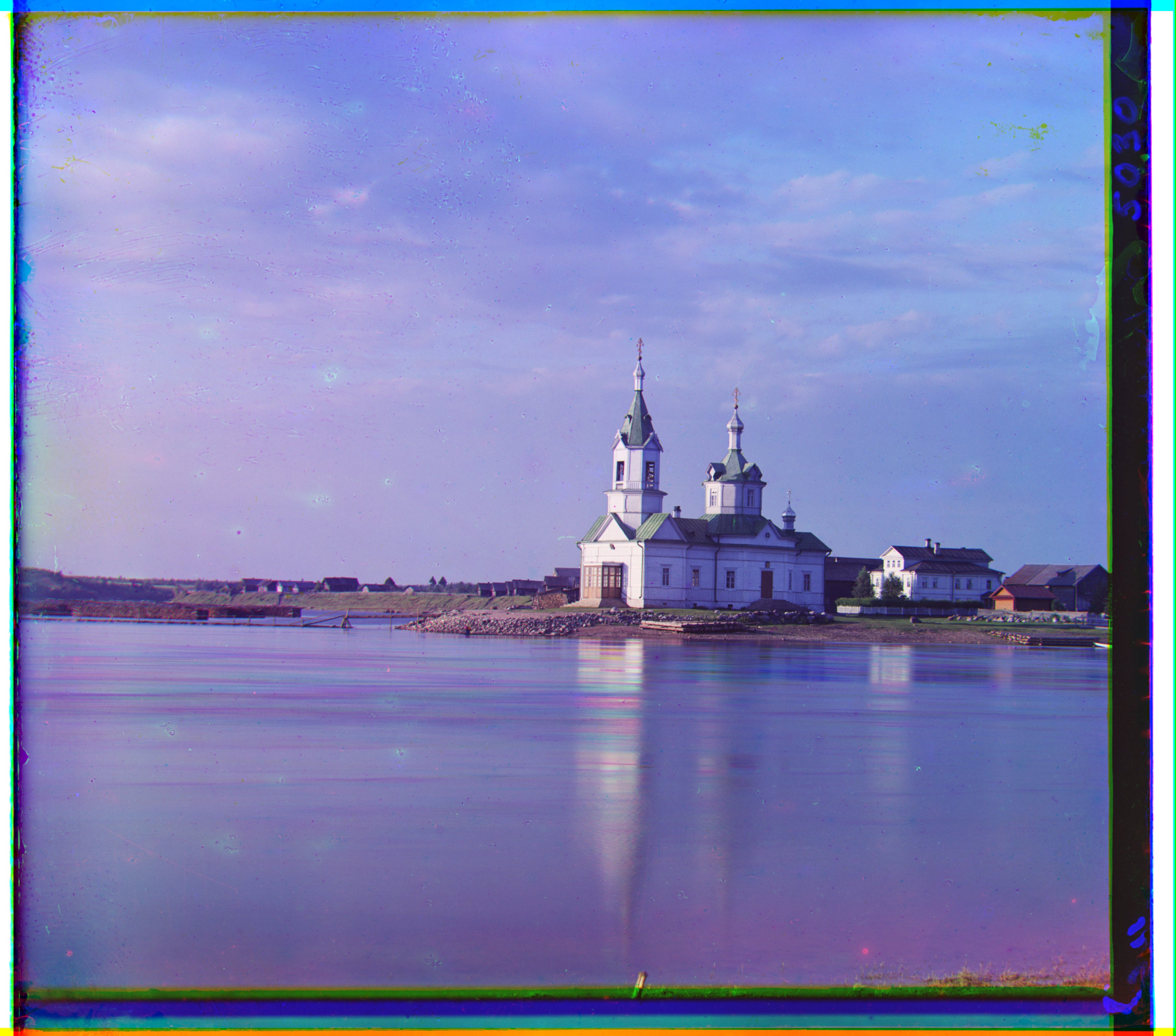
Results (Aligned RGB, high‑res TIFF, pyramid)
Outputs produced on the high‑resolution TIFFs using the coarse‑to‑fine alignment and per‑channel min–max rendering.


Alignment Offsets and Compute Times (Combined L2 + NCC)
| Image | B→G shift | R→G shift | Total time (s) |
|---|---|---|---|
| cathedral | up 5 px, left 2 px | down 7 px, right 1 px | 0.388 |
| church | up 25 px, left 4 px | down 33 px, left 8 px | 30.243 |
| emir | up 49 px, left 22 px | down 57 px, right 18 px | 30.524 |
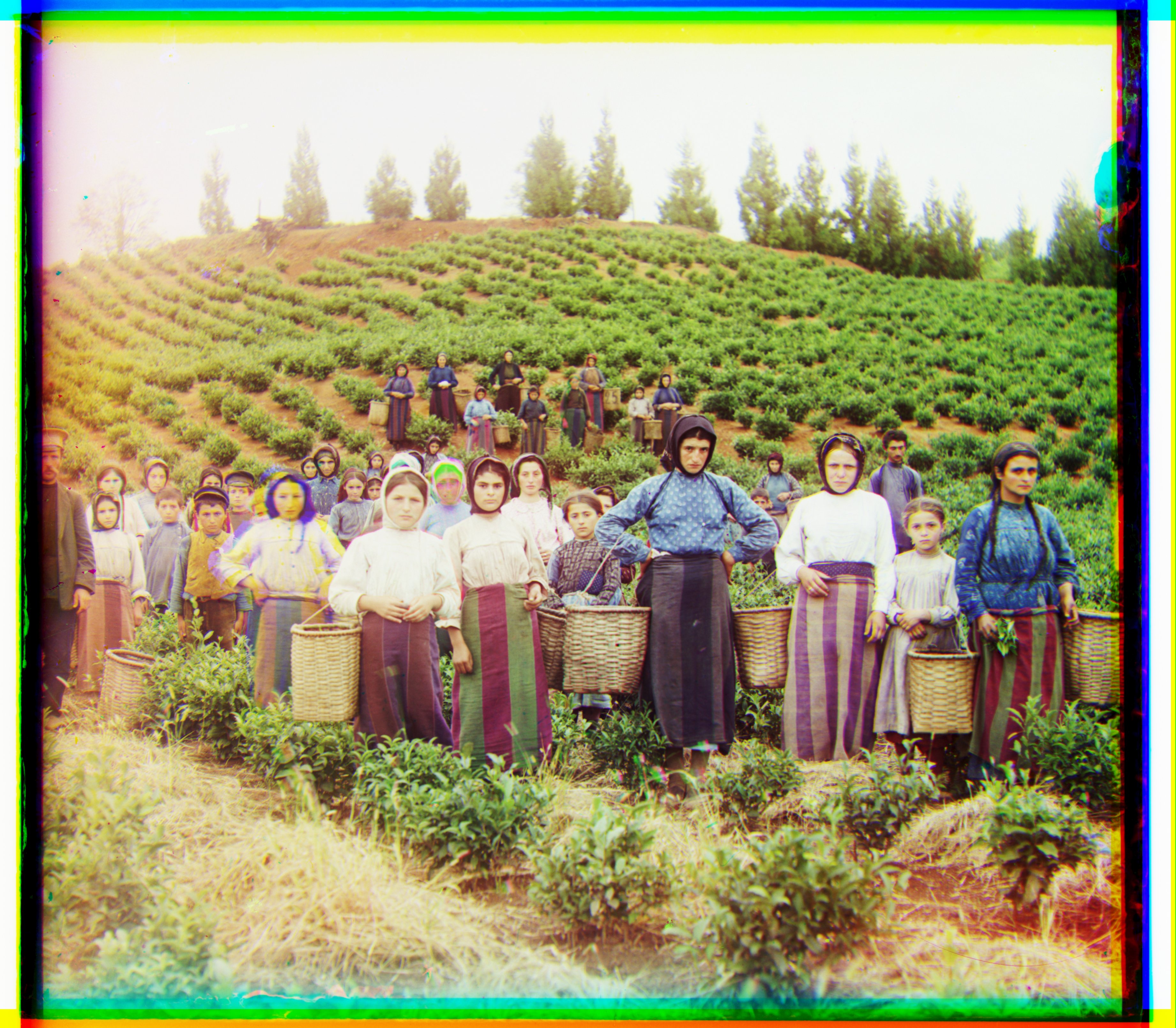
| harvesters | up 59 px, left 16 px | down 64 px, left 2 px | 30.019 |
| icon | up 39 px, left 17 px | down 48 px, right 5 px | 30.702 |
| italil | up 38 px, left 21 px | down 39 px, right 15 px | 30.655 |
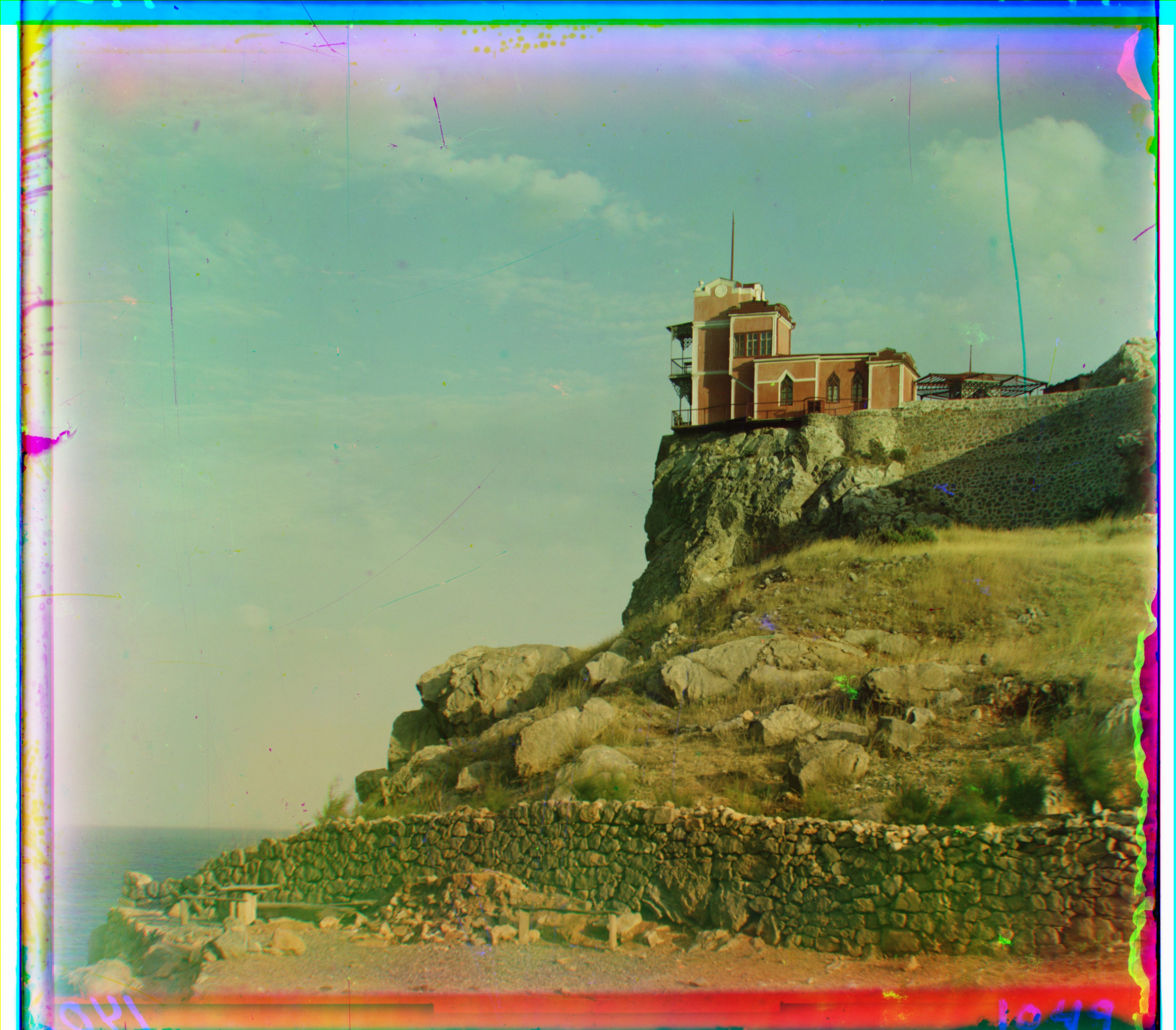
| lastochikino | down 2 px, right 2 px | down 78 px, left 7 px | 30.435 |
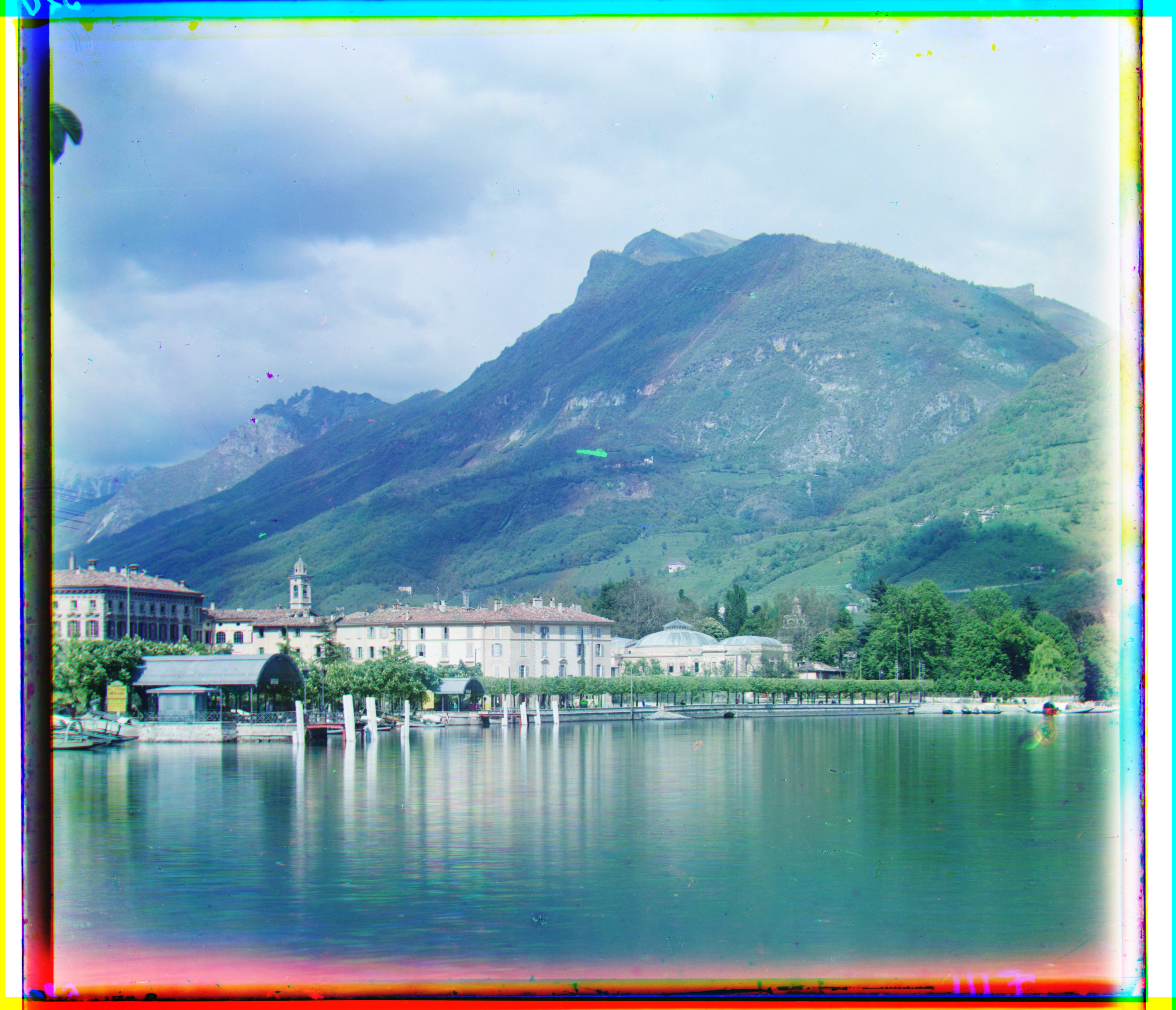
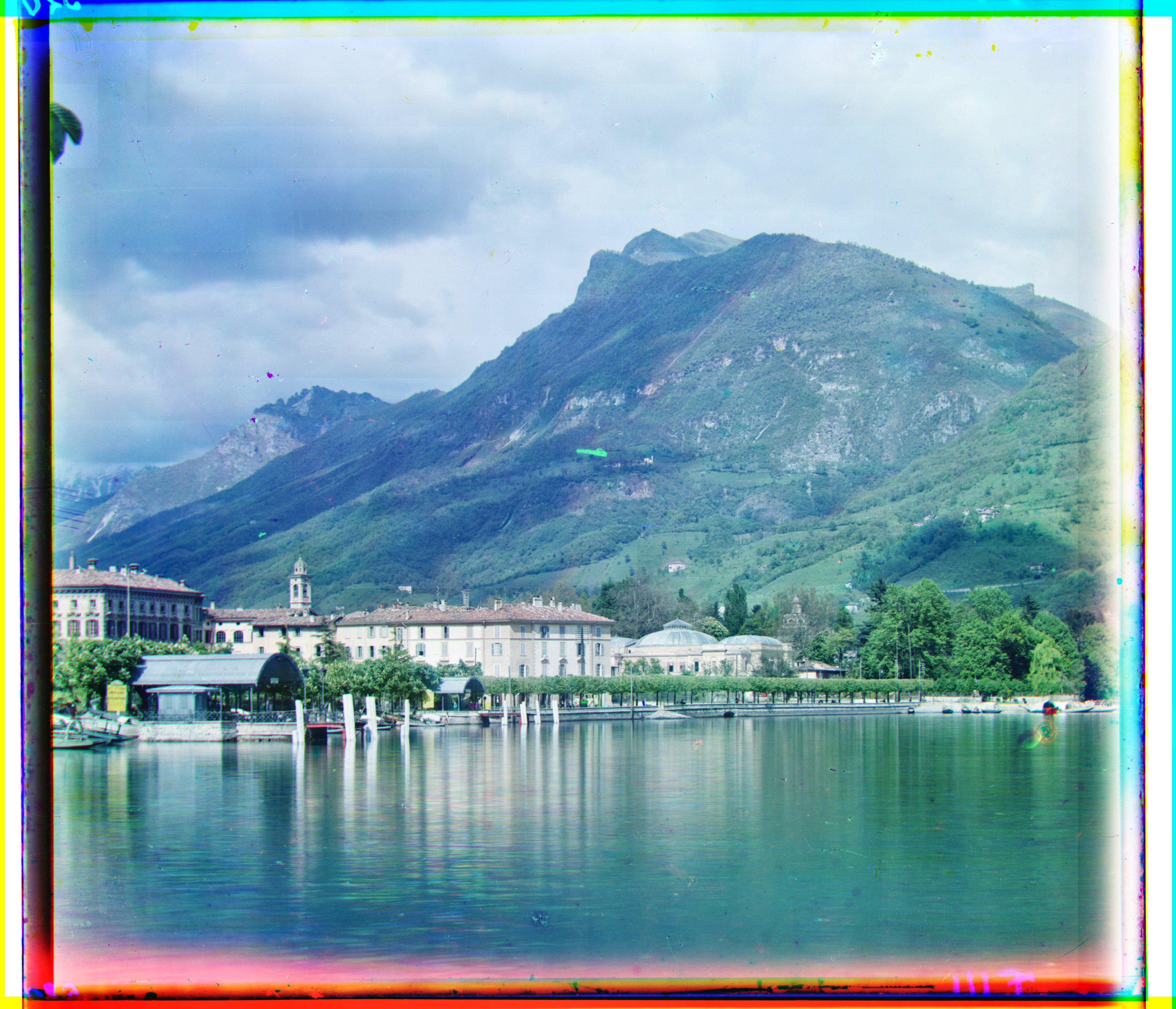
| lugano | up 40 px, right 15 px | down 53 px, left 13 px | 30.780 |
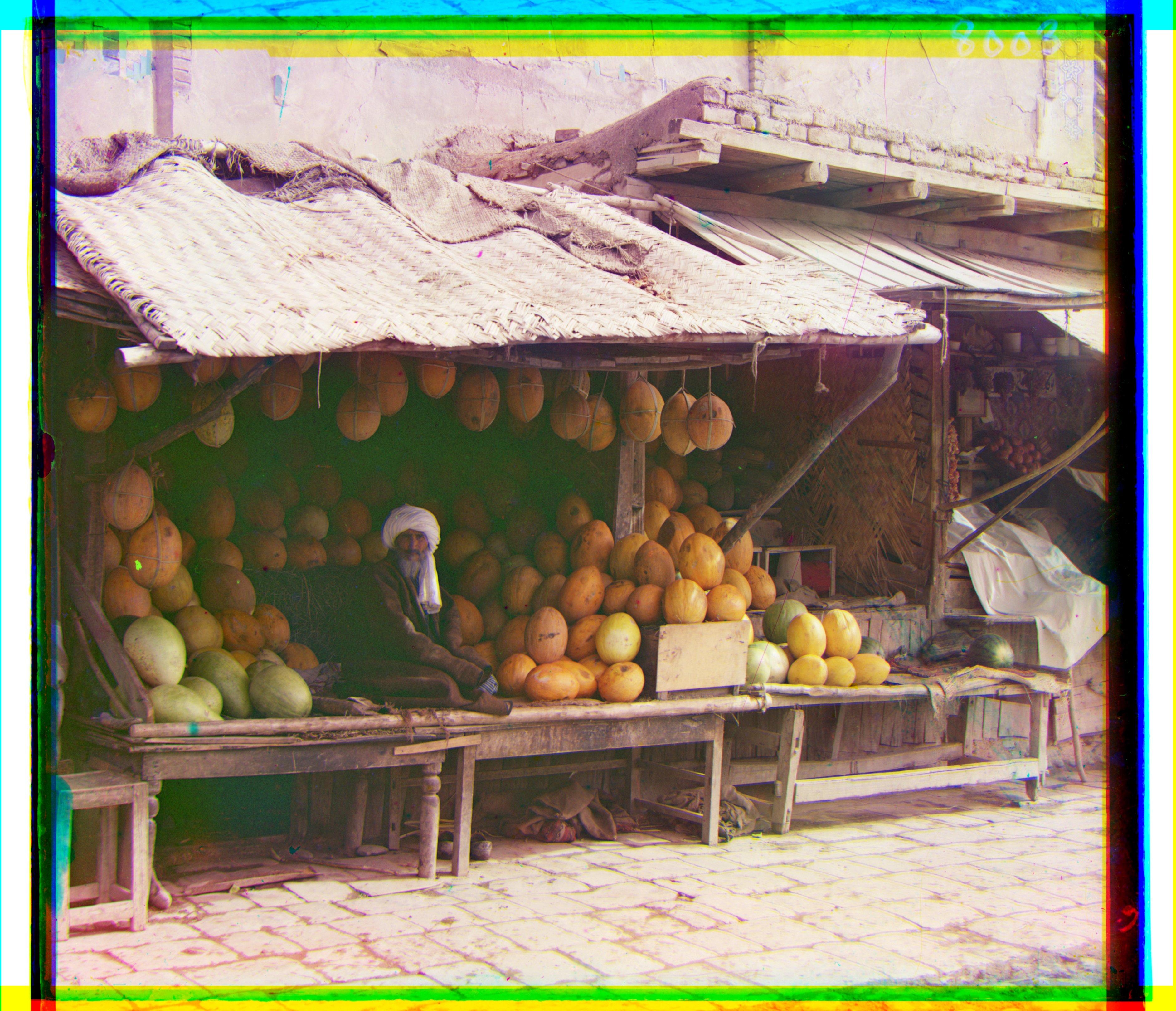
| melons | up 81 px, left 10 px | down 96 px, right 4 px | 31.156 |
| monastery | down 3 px, left 2 px | down 6 px, right 1 px | 0.377 |
| self_portrait | up 78 px, left 29 px | down 98 px, right 8 px | 30.837 |
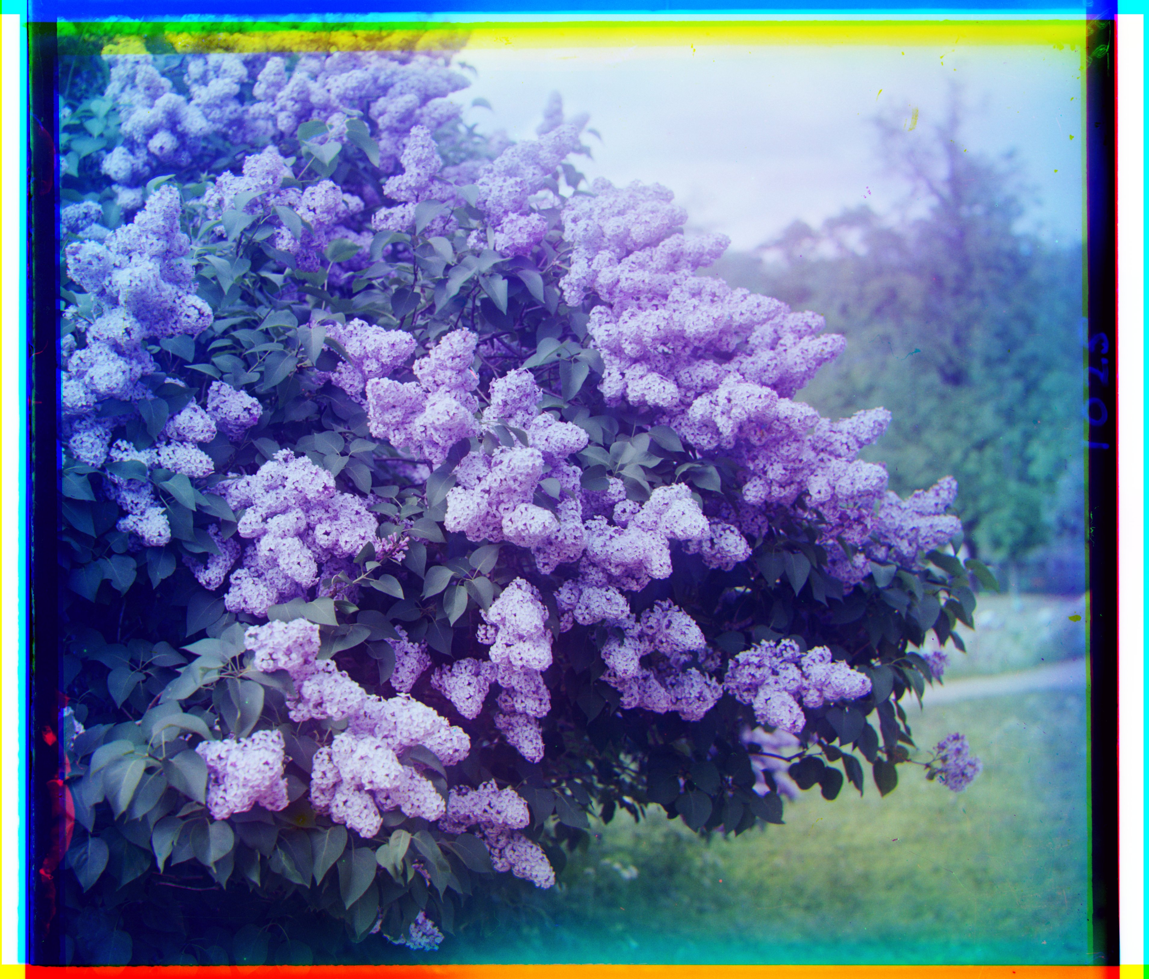
| siren | up 48 px, right 6 px | down 47 px, left 18 px | 32.307 |
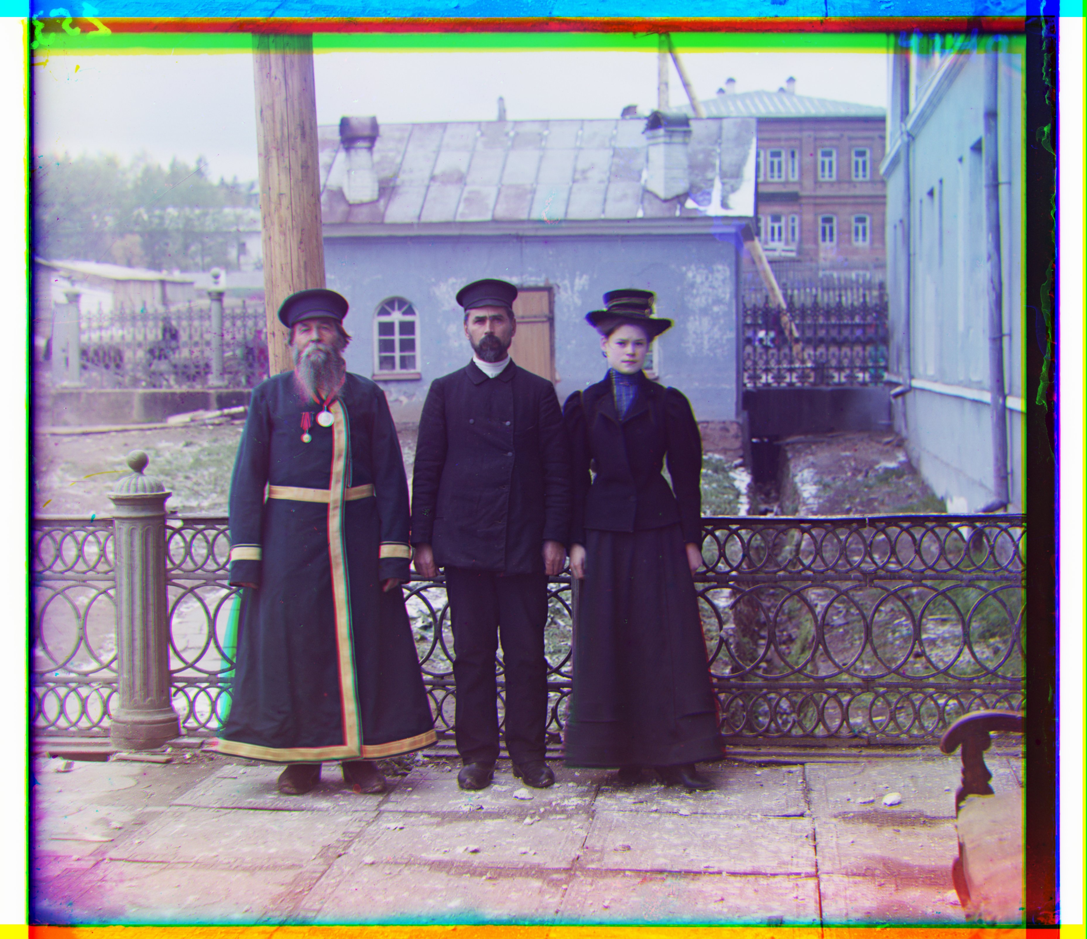
| three_generations | up 50 px, left 15 px | down 58 px, left 4 px | 30.443 |
| tobolsk | down 3 px, left 3 px | down 4 px | 0.387 |
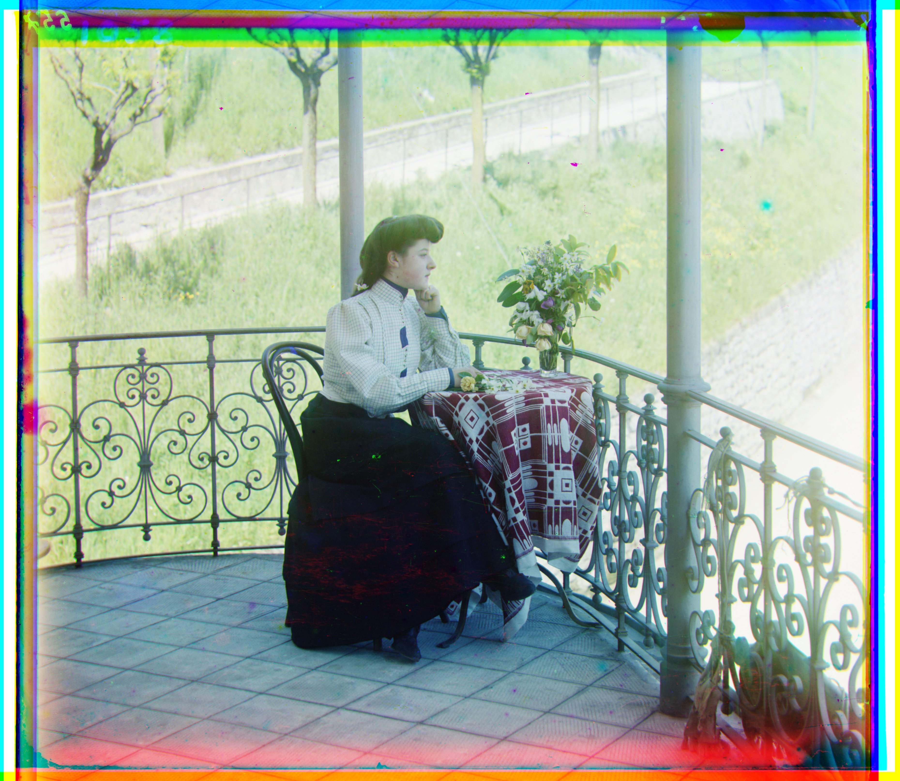
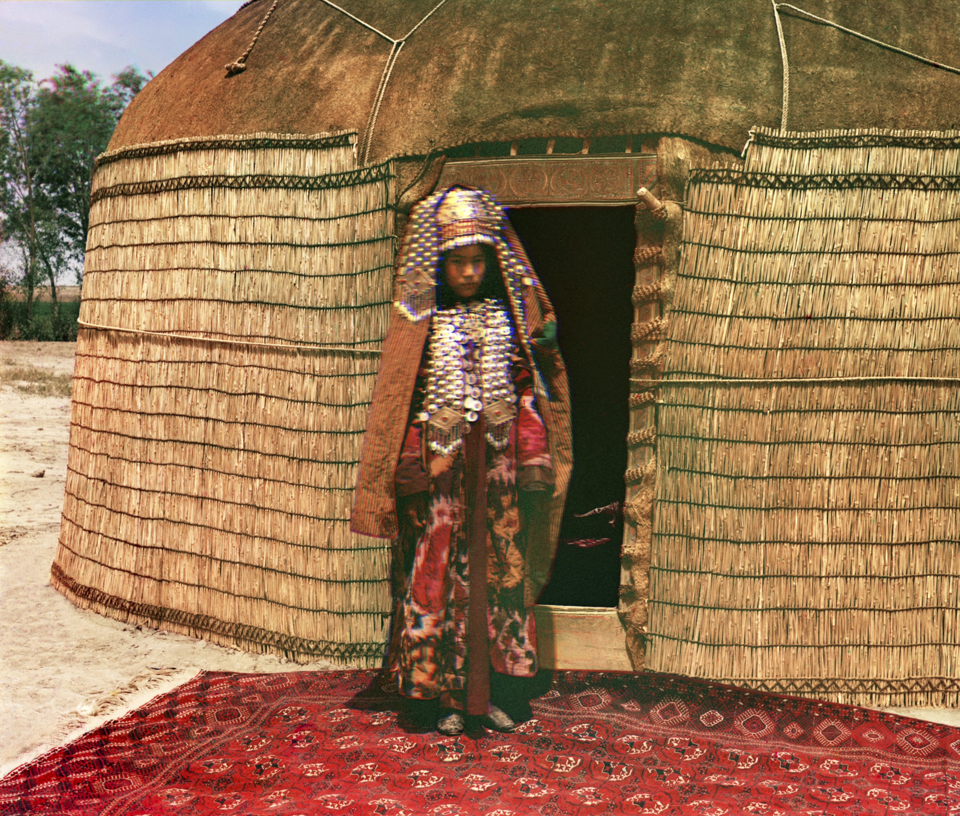
Additional Results — Prokudin‑Gorskii Collection (my selections)
Bells & Whistles Results
Below are result summaries for each enhancement, with brief approach notes and before/after comparisons.
Automatic cropping
Intuition: Real borders sit at the edges, look like long straight lines, and contain lots of extreme pixels — very bright (white) and very dark (black). In contrast, real scene content has mixed mid‑tones and broken/curvy edges; full rows or columns in the interior are rarely dominated by extremes, which makes border lines easy to spot.
Method:
- Scan full lines: For left/right, examine vertical lines (columns) spanning the full height; for top/bottom, examine horizontal lines (rows) spanning the full width.
- Classify pixels: Mark a pixel as black if ≤ BLACK_THR and white if ≥ WHITE_THR. Thresholds are auto‑estimated from a thin outer strip when enabled, otherwise use WHITE_THR ≈ 0.85 and BLACK_THR ≈ 0.22.
- Score each line: Compute the fraction of pixels on that line that are extreme (black or white). If the fraction ≥ 70%, classify that line as border.
- Step inward robustly: Move inward while there is 4‑of‑5 neighbor agreement that consecutive lines are border (reduces noise/outliers).
- Safety cap: Never crop more than 45% from any side, and do this per channel (B/G/R) to avoid color bias.
As visible below, applying the procedure independently to each channel (B/G/R) produces consistently good crop boxes.
Limitation: in some cases, adjacent strong whites and blacks can blend (e.g., via blur/compression/downsampling) into gray along a line, weakening the extreme‑pixel signal and causing under‑detection of borders. The 4‑of‑5 neighbor voting and per‑channel processing help, but are not perfect; tightening thresholds or the extreme‑fraction can further improve those edge cases.
Automatic contrasting
Motivation
Global methods (min–max scaling or vanilla histogram equalization) can either leave low‑contrast regions flat or push highlights/shadows too far. Many Prokudin‑Gorskii images have locally varying illumination; we need a method that enhances texture and structure region‑by‑region without amplifying noise or creating halos.
Approach
- What it is: Contrast Limited Adaptive Histogram Equalization (CLAHE) boosts local contrast using small tiles and clipped histograms.
- Why histograms help: A histogram is a simple bar chart of how many pixels have each brightness (0–255). If most bars sit in a narrow range (e.g., mostly dark), the tile looks flat; spreading tones out across the range reveals hidden detail without changing the scene.
- Color space: Convert the image to LAB and operate on the L (luminance) channel only; A/B (color) channels are left unchanged and merged back after equalization to preserve hues.
- How it works:
- Divide into tiles: Split the image into an N×N grid (configurable; e.g., 24×24 here).
- Build a histogram: For each tile, count pixels at each brightness (0–255). This shows how tones are distributed.
- Clip tall bins: Set a per‑bin threshold as T × (average count per bin) (with T ≈ 2.0). Cap bars above this level and redistribute the excess uniformly to avoid over‑amplifying noise or small peaks.
- Equalize via CDF: The CDF is a running total of the histogram; for any brightness x it tells you what fraction of pixels in this tile are ≤ x. We map x → CDF(x) (normalized to 0–1), so darkest values go near 0, brightest near 1, and crowded ranges are spread out — revealing detail and increasing local contrast.
- Blend between tiles: Each tile yields its own remapping curve. For pixels near tile borders, we take the four surrounding tiles’ curves and combine them with bilinear weights based on the pixel’s relative (x,y) position (weights sum to 1). The pixel is remapped by this weighted average, which removes visible seams between tiles.
- Luminance‑only: Equalization is applied to the L channel, then converted back to BGR; this preserves color fidelity while enhancing local detail.
- Trade‑offs: Larger tiles → smoother, more global look; smaller tiles → stronger local contrast but risk amplifying noise if T is too high.
Before & After Results

The enhanced versions breathe noticeably more contrast and clarity, giving a crisper, more lifelike appearance; by comparison, the originals feel slightly soft and subdued.
Automatic white balance
Motivation
Channels often have different gains/illumination, leading to color casts (e.g., blue/green tint). We aim to estimate a neutral illuminant and re-scale channels so neutrals appear gray/white.
Approach
Gray‑World algorithm. Intuition: under a neutral illuminant, the spatial average of an image should be achromatic (gray). If an image has a color cast, the per‑channel means differ; we correct this by scaling each channel so their means match a common gray target.
- Compute means: \(\mu_R,\ \mu_G,\ \mu_B\) over interior pixels (optionally exclude borders/outliers).
- Choose gray target: I use the average of the channel means, \(\mu_{\text{target}} = (\mu_R + \mu_G + \mu_B)/3\).
- Scale channels: apply gains \(s_c = \mu_{\text{target}} / \mu_c\) to each channel \(c \in \{R,G,B\}\), then clip to the display range.
This neutralizes global color casts while preserving relative contrasts; using interior pixels and clipping avoids bias from borders and outliers.
Implementation note: I used the average-of-means gray target \(\mu_{\text{target}} = (\mu_R+\mu_G+\mu_B)/3\) (not a fixed 0.5), and clipped per-channel gains to a safe range before applying them.
Before & After Results

Assuming the Emir’s hat and the church facade are meant to be white, the Gray‑World correction makes these regions appear white in the new images—whereas they showed clear color casts in the originals.
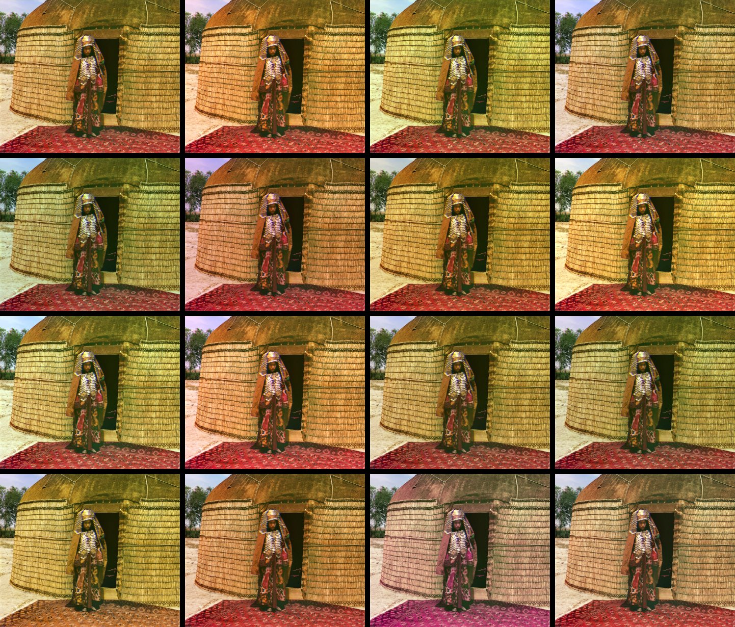
Better color mapping
Motivation
Channel gains and spectral responses can differ; simple per‑channel scaling (white balance) may not fully capture cross‑channel interactions. I explored small color transforms to find a mapping that looks most realistic.
Approach
I generated a small set of candidates using two tiny 3×3 matrix families — diagonal channel gains and cross‑channel mixing — then picked the most natural‑looking result.
- Color basis (additive RGB): Red + Green = Yellow (warm), Green + Blue = Cyan (cool), Red + Blue = Magenta. Scaling channels nudges colors along these axes.
- Diagonal gains (warm RG+, cool BG+, magenta RB+): Multiply channels independently (diagonal matrix). For example:
- RG+: boost R and G slightly (~0.28) → warmer/yellowish look.
- BG+: boost B and G → cooler/cyan look.
- RB+: boost R and B → magenta tint.
- Cross‑channel mixes: Add a small fraction ε ≈ 0.25 from one channel into another (off‑diagonal entries). Example: B' = (1−ε)·B + ε·G shifts blue slightly toward cyan, reducing magenta casts; similarly R' ← R + ε·G, G' ← G + ε·B, etc.
- Baselines: Diagonal gray‑world and white‑patch gains for reference.
- Evaluation: Render candidates to sRGB, size‑match, and lay out in a grid to judge realism (skin tones, skies, foliage) side‑by‑side.
Note: these mappings are not universal. The most natural‑looking transform is image‑dependent (scene/illuminant) and therefore relative; the grid enables per‑image selection rather than a single fixed mapping.
Chosen mapping (bottom‑right tile)
I picked the bottom‑right tile of the grid as the final mapping. This corresponds to a subtle blue‑from‑green mix:
Intuition: adding a touch of green into blue reduces residual magenta casts and improves foliage/sky balance without over‑saturating reds.
Grid and comparison (tippie)

The mapped image (right) looks more realistic and less like a warm filter is applied (as the left side feels). The sand color also appears more natural.
Better features
Gradient-based approach
Intuition: edges are places where neighboring pixels differ strongly. Compute horizontal and vertical finite differences, then combine them into a gradient magnitude and normalize. This captures structure while being less sensitive to absolute brightness.
- Computation: For each channel independently, apply the finite differences above, form the magnitude, min–max to [0,1] if needed, then z‑normalize (zero mean, unit variance).
- Why it helps: Gradients emphasize shared structure across channels while down‑weighting absolute intensity/gain differences.
Alignment
For each candidate shift, I evaluate equal‑weight NCC and L2 on the gradient maps and pick the best shift in a coarse‑to‑fine pyramid (same window schedule as before).
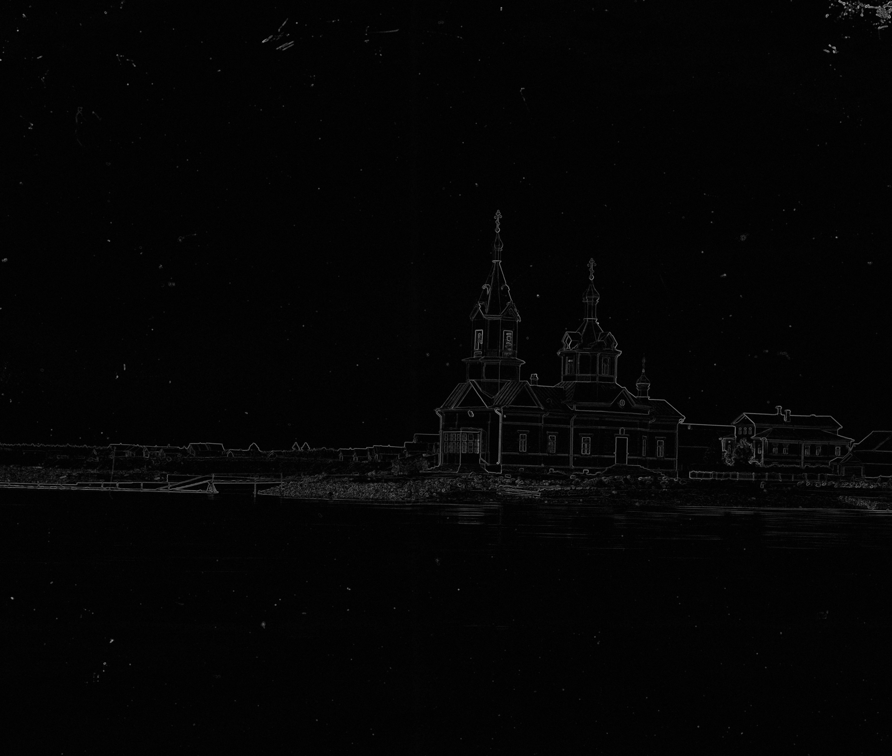
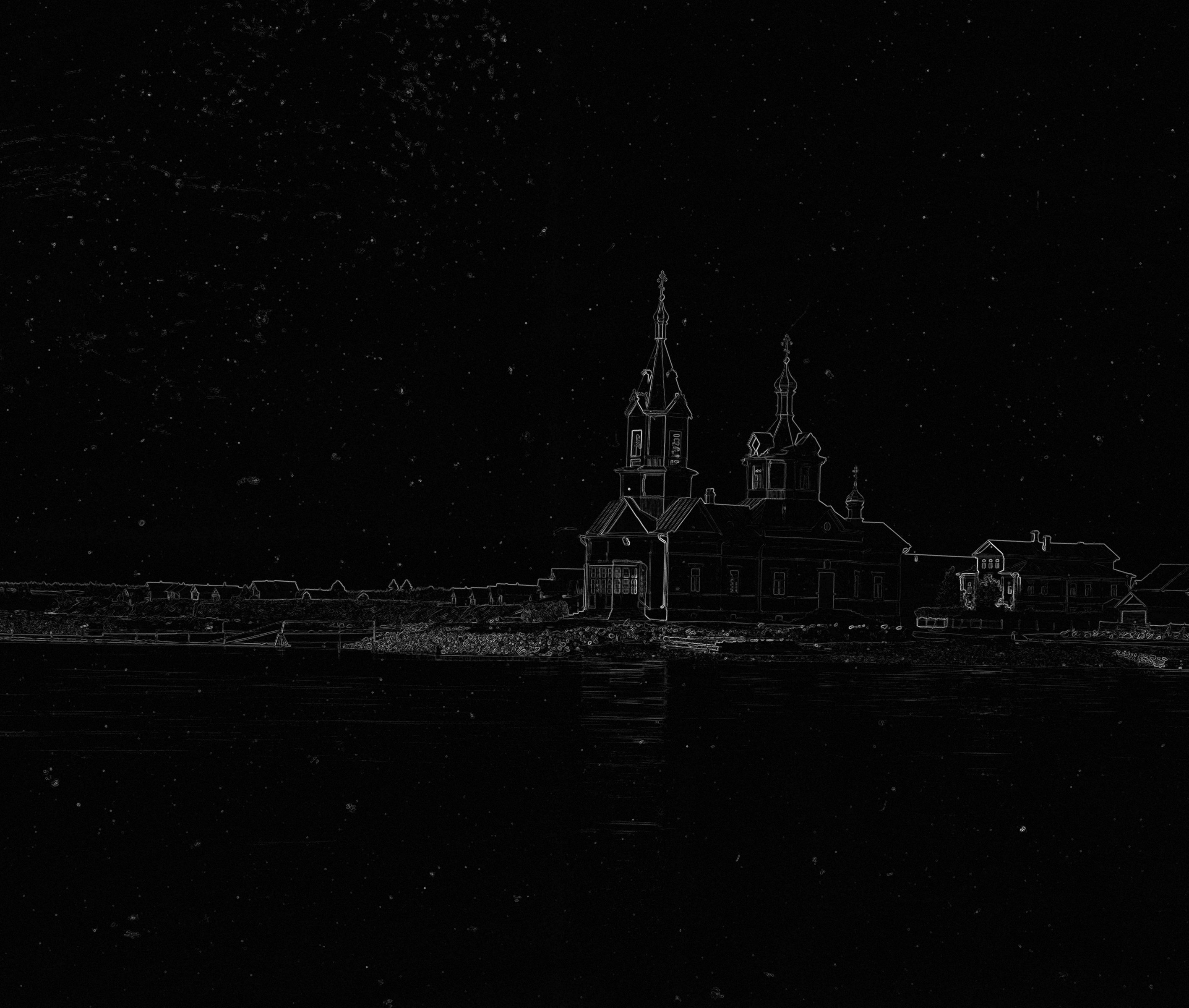
These gradient maps are used directly for alignment: the algorithm aligns on gradients (not raw intensities) using equal‑weight NCC and L2.
Finding: On this dataset, gradients+NCC/L2 did not outperform the prior method in a significant way, but it was a useful experiment that confirmed alignment robustness to brightness changes.