Project 3
CS180/280A: Intro to Computer Vision and Computational Photography
Image Warping and Mosaics


A.1: Shoot and Digitize Pictures
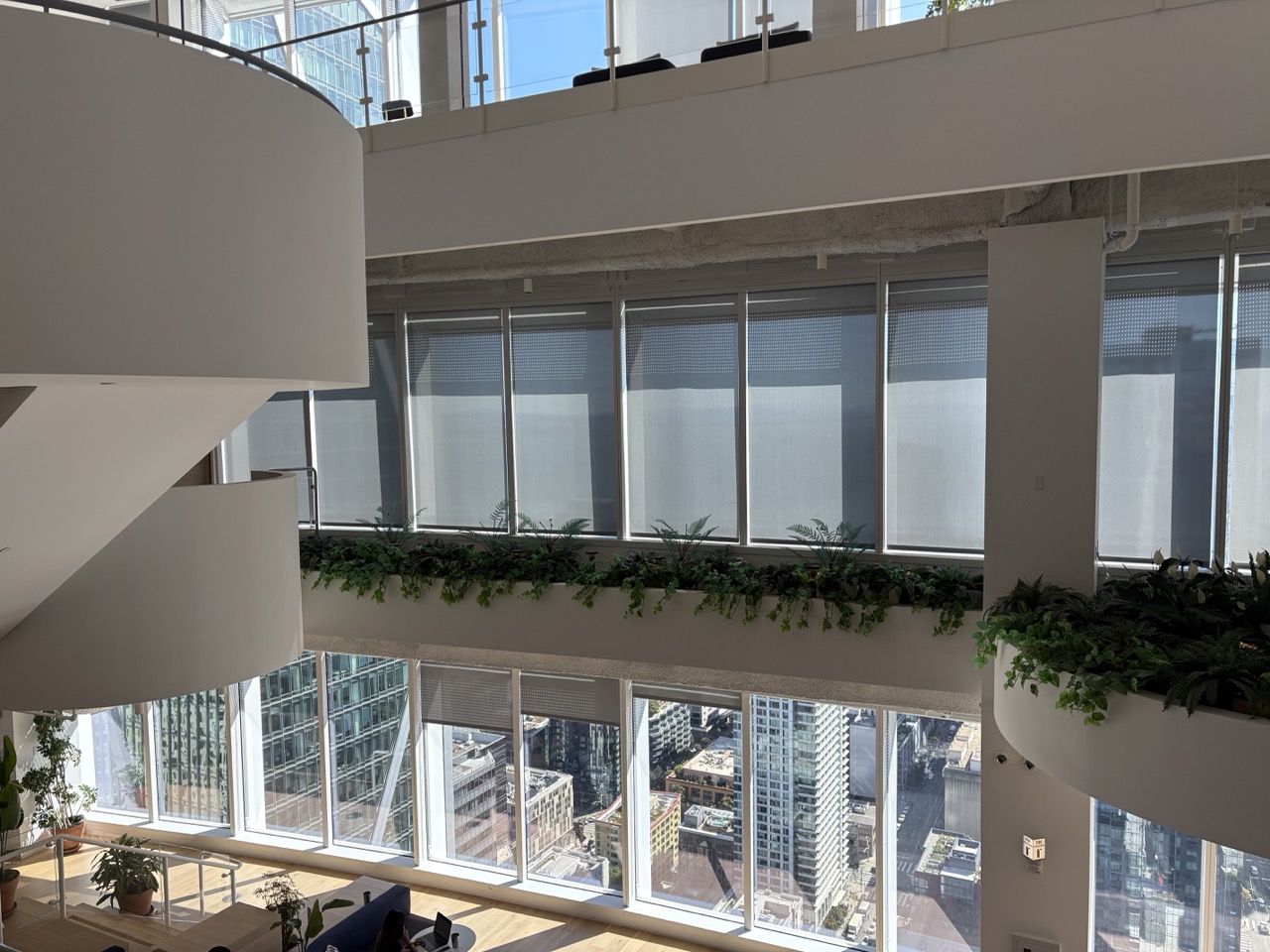
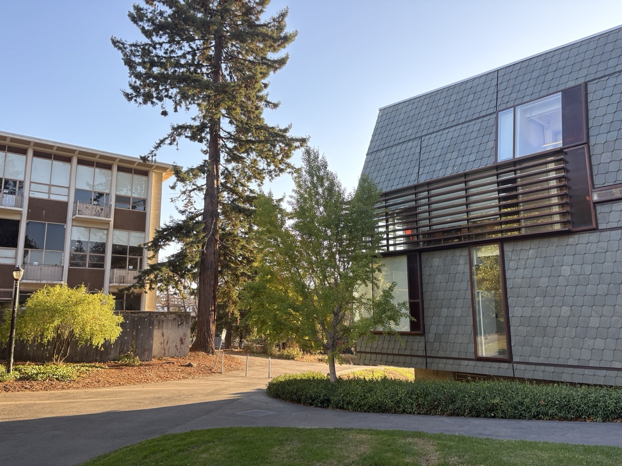
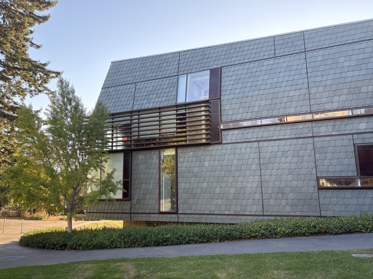
I captured each set to induce projective (perspective) transforms by fixing the center of projection and rotating the camera. Photos were taken on an iPhone 16 using AE/AF LOCK (press-and-hold) to keep exposure and focus constant, which later helps produce clean mosaics.
Set 1 — Music Library (campus)
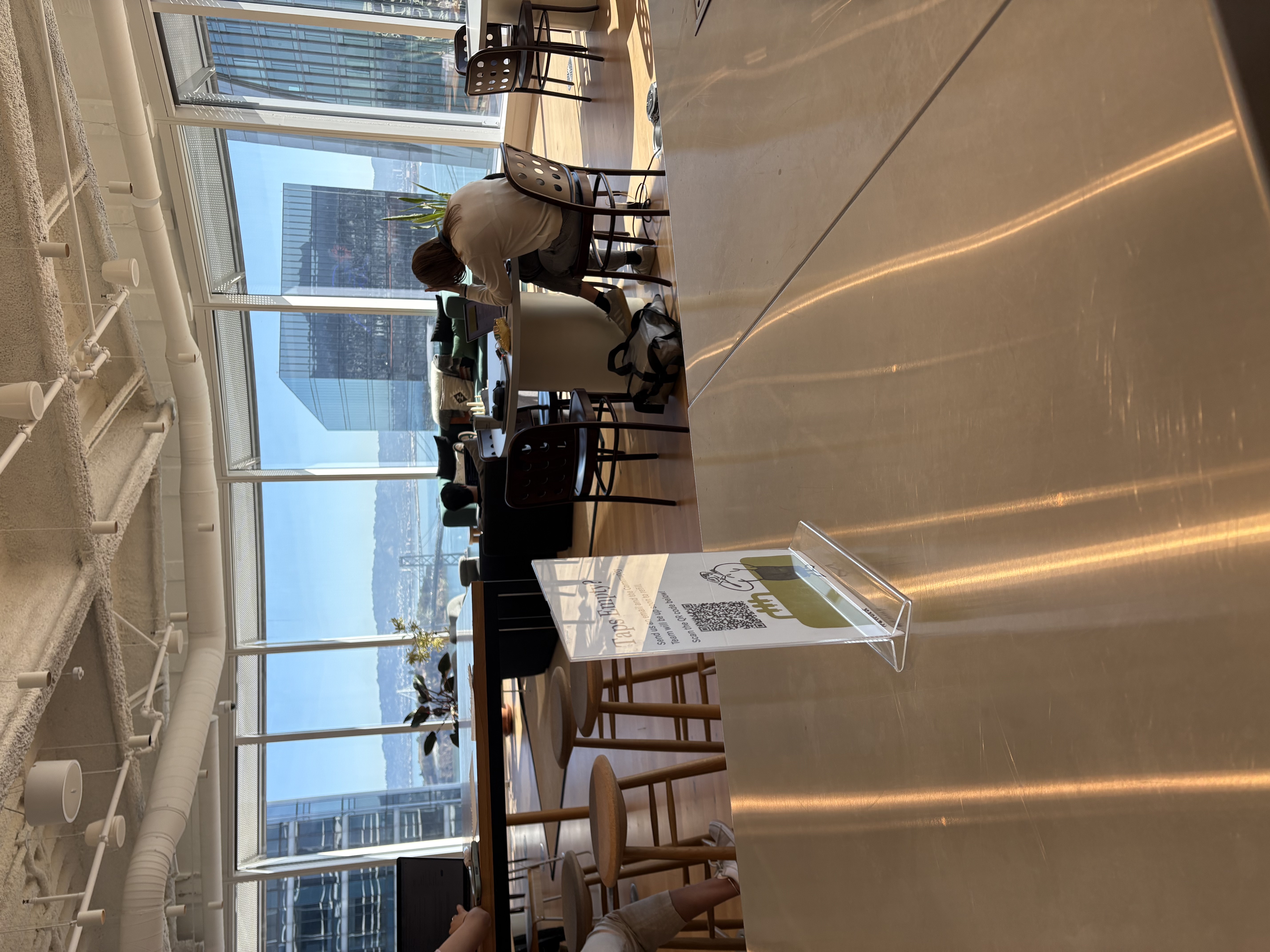
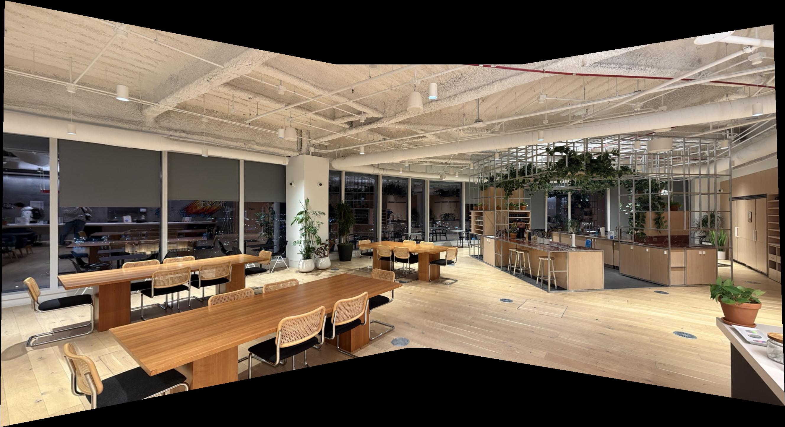
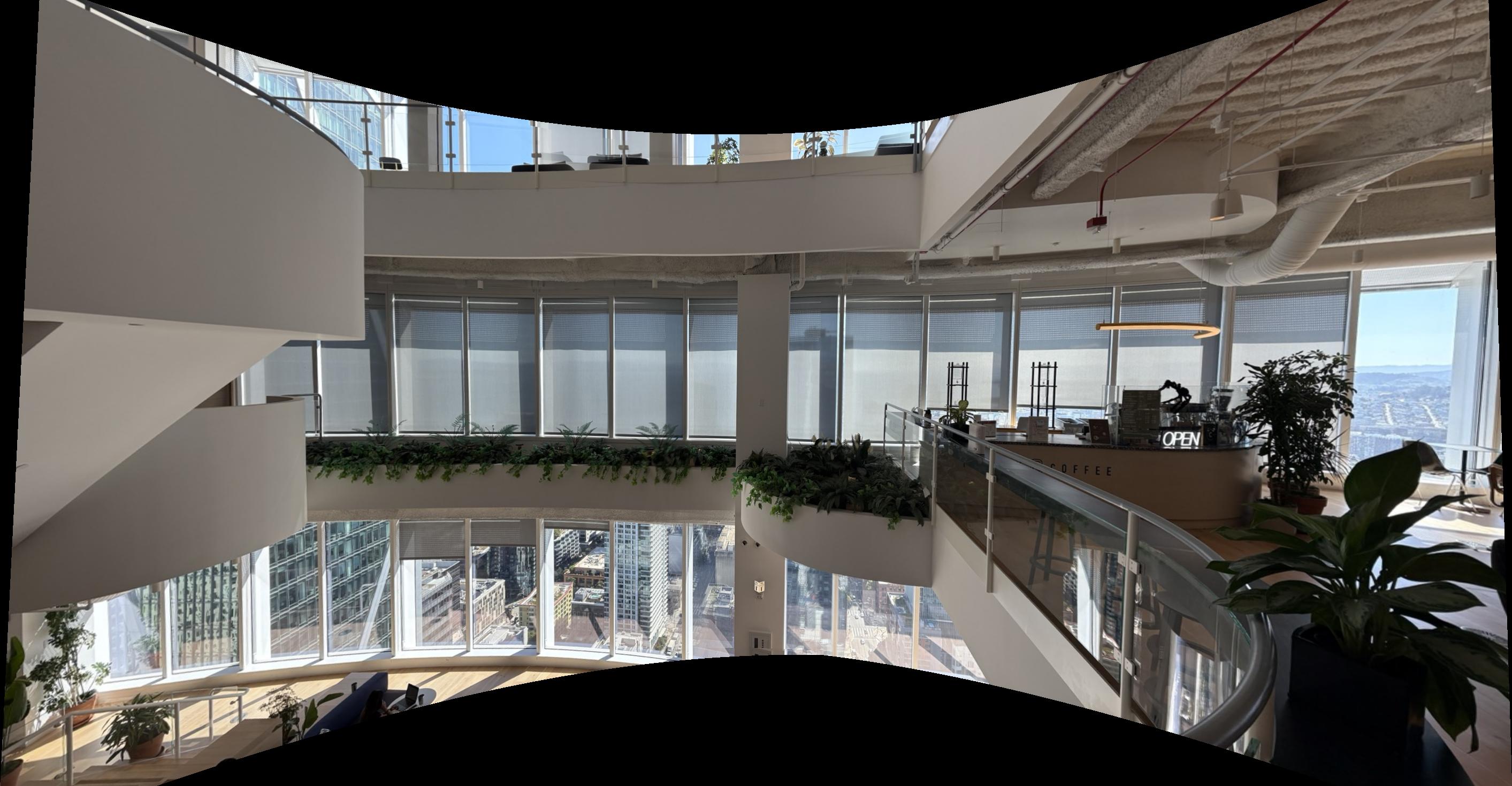
Set 2 — WeWork, Salesforce Tower (SF)

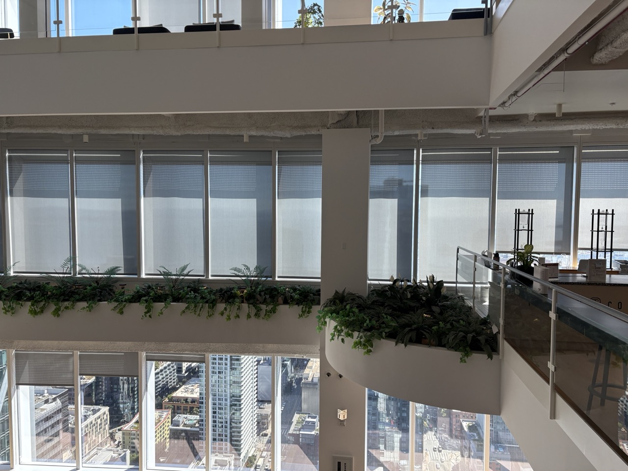
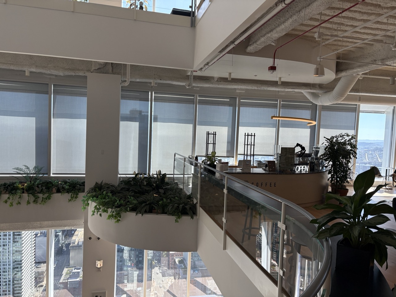
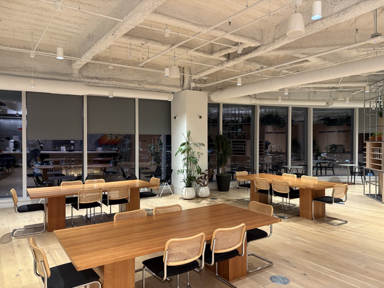
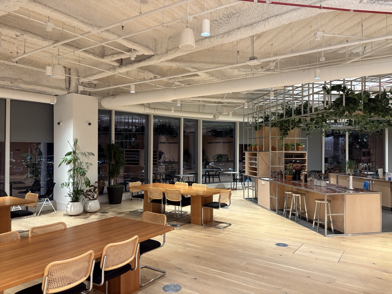
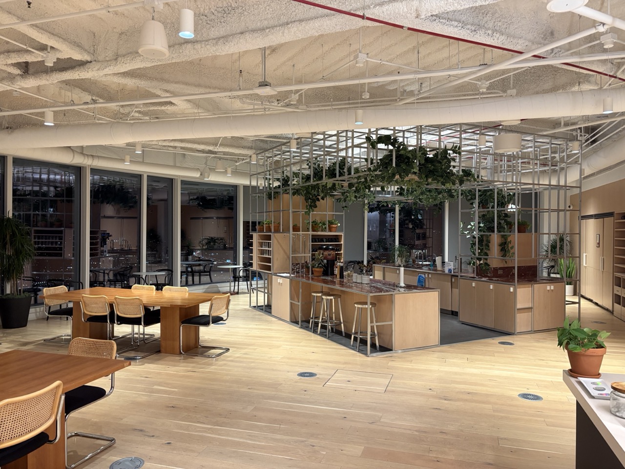
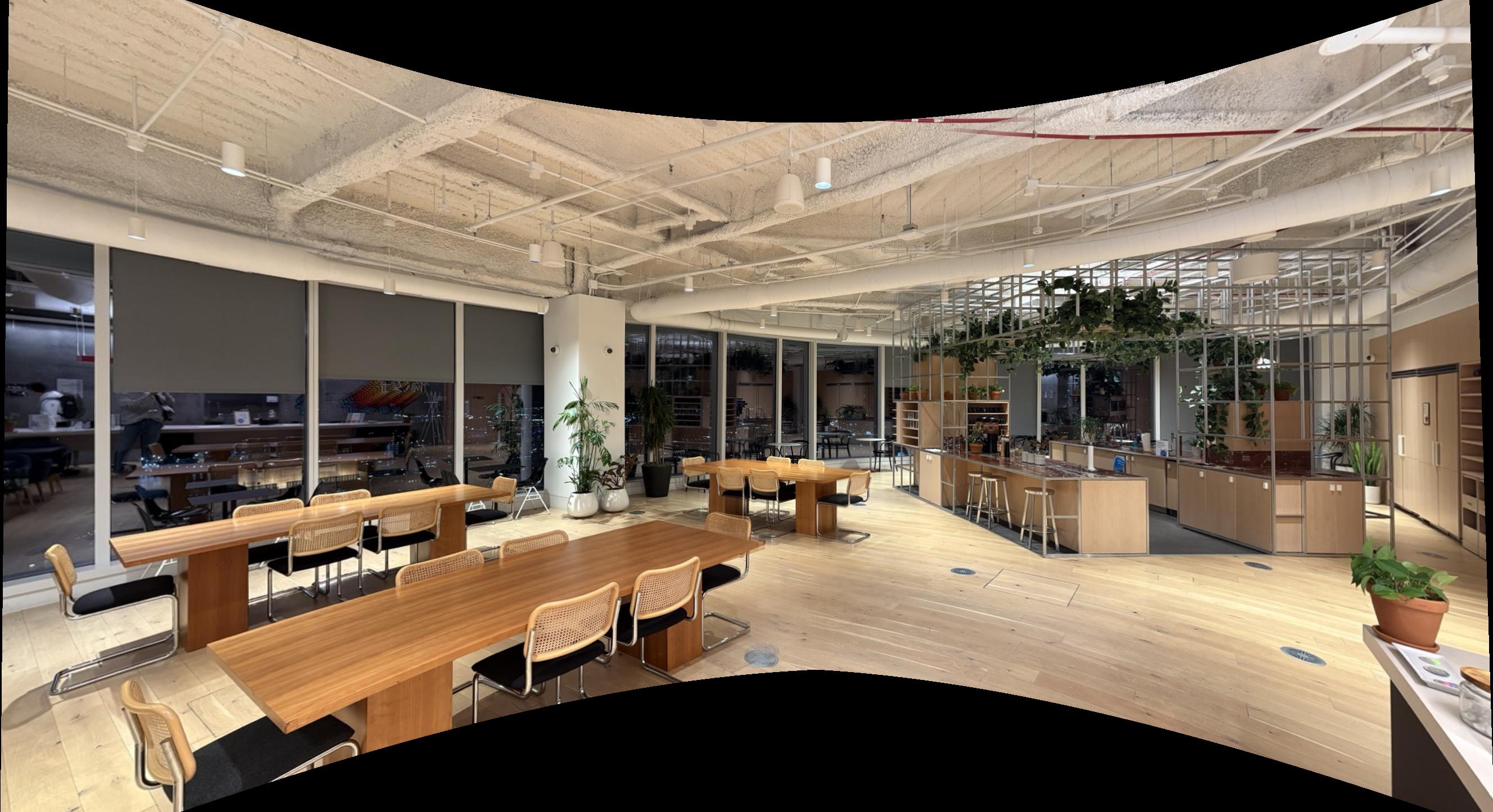
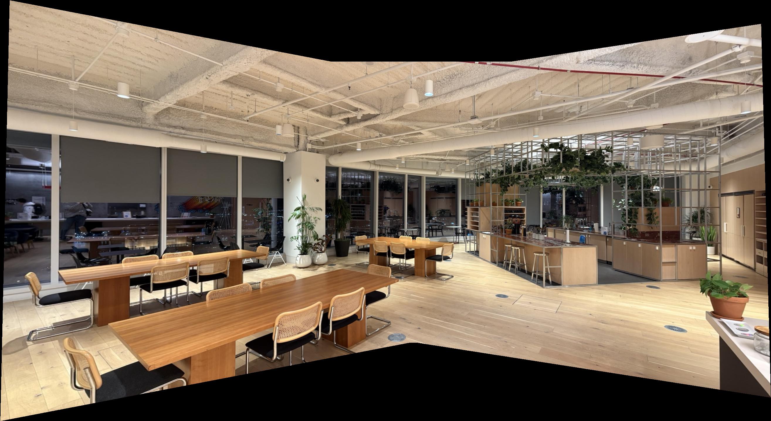
Set 3 — WeWork, Salesforce Tower (SF)

A.2: Recover Homographies
General idea
Using point correspondences between two images, we can solve for the projective transform matrix H that warps pixels from one image plane to the other.
Derivation
Consider corresponding pixel coordinates \((x_i, y_i)\) in image 1 and \((x'_i, y'_i)\) in image 2. With a camera rotation (or a planar scene), the two views are related by a planar projective transform (homography) between their image planes. We reason in projective space by fixing the common image plane at \(z=1\) and using homogeneous coordinates: \(\mathbf{a}_i=[x_i\;y_i\;1]^\top\) and \(\mathbf{b}_i=[x'_i\;y'_i\;1]^\top\), each defined up to scale. A homography \(H\) maps viewing rays between the planes: \(\tilde{\mathbf{b}}_i \sim H\,\tilde{\mathbf{a}}_i\). In coordinates we write \[ \mathbf{b}_i \;=\; H\,\mathbf{a}_i,\qquad \mathbf{a}_i = [x_i\; y_i\; 1]^\top,\;\; \mathbf{b}_i = [x'_i\; y'_i\; 1]^\top. \] \[ \begin{bmatrix} x'_i\\[2pt] y'_i\\[2pt] 1 \end{bmatrix} = \begin{bmatrix} h_{11} & h_{12} & h_{13}\\ h_{21} & h_{22} & h_{23}\\ h_{31} & h_{32} & h_{33} \end{bmatrix} \begin{bmatrix} x_i\\[2pt] y_i\\[2pt] 1 \end{bmatrix}. \] We rescale the vector to recover image coordinates by dividing the first two components by the third (\(z\)): \(x \leftarrow x/z\), \(y \leftarrow y/z\). This yields the standard form \[x'_i = \frac{h_{11}x_i + h_{12}y_i + h_{13}}{h_{31}x_i + h_{32}y_i + h_{33}},\qquad y'_i = \frac{h_{21}x_i + h_{22}y_i + h_{23}}{h_{31}x_i + h_{32}y_i + h_{33}}.\]Solving for H
Because the model is defined only up to a global scale (multiplying all \(h_{jk}\) by the same constant leaves the mapping unchanged), we can fix h to \(h_{33}=1\). This leaves us with only 8 unknowns. Rearranging each correspondence results in two linear equations: \[ x'_i\big(h_{31}x_i + h_{32}y_i + 1\big) = h_{11}x_i + h_{12}y_i + h_{13},\qquad y'_i\big(h_{31}x_i + h_{32}y_i + 1\big) = h_{21}x_i + h_{22}y_i + h_{23}. \]Rearranged to be linear in the unknowns:
\[
x_i h_{11} + y_i h_{12} + h_{13} - x'_i x_i h_{31} - x'_i y_i h_{32} = x'_i,\qquad
x_i h_{21} + y_i h_{22} + h_{23} - y'_i x_i h_{31} - y'_i y_i h_{32} = y'_i.
\]
\[\big[\,x_i\ y_i\ 1\ 0\ 0\ 0\ -x_ix'_i\ -y_ix'_i\,\big]\\,\mathbf{h} = x'_i,\qquad
\big[\,0\ 0\ 0\ x_i\ y_i\ 1\ -x_iy'_i\ -y_iy'_i\,\big]\\,\mathbf{h} = y'_i,\]
with \(\mathbf{h}=[h_{11},h_{12},h_{13},h_{21},h_{22},h_{23},h_{31},h_{32}]^\top\). Stacking over all points gives \(A\mathbf{h}=\mathbf{b}\), which we can then solve solve with least squares.
Examples
Correspondences
Correspondences were selected manually by clicking distinctive points across the image pairs to precisely align pixels before estimating the homography.
Linear system and recovered H
\[
\underbrace{\begin{bmatrix}
1195 & 175 & 1 & 0 & 0 & 0 & -897445 & -131425 \\
0 & 0 & 0 & 1195 & 175 & 1 & -280825 & -41125 \\
1025 & 230 & 1 & 0 & 0 & 0 & -628325 & -140990 \\
0 & 0 & 0 & 1025 & 230 & 1 & -266500 & -59800 \\
780 & 223 & 1 & 0 & 0 & 0 & -296400 & -84740 \\
0 & 0 & 0 & 780 & 223 & 1 & -165360 & -47276 \\
1059 & 324 & 1 & 0 & 0 & 0 & -675642 & -206712 \\
0 & 0 & 0 & 1059 & 324 & 1 & -370650 & -113400 \\
\vdots & \vdots & \vdots & \vdots & \vdots & \vdots & \vdots & \vdots
\end{bmatrix}}_{A}
\cdot
\underbrace{\begin{bmatrix}
h_{11}\\ h_{12}\\ h_{13}\\ h_{21}\\ h_{22}\\ h_{23}\\ h_{31}\\ h_{32}
\end{bmatrix}}_{h}
=
\underbrace{\begin{bmatrix}
751\\ 235\\ 613\\ 260\\ 380\\ 212\\ 638\\ 350\\ \vdots
\end{bmatrix}}_{b}
\]
Recovered homography matrix (from JSON)
\[
H\;\approx\;
\begin{bmatrix}
1.91953 & -0.109304 & -881.483100 \\
0.436998 & 1.576739 & -362.117488 \\
0.000719554 & -0.0000300114 & 1
\end{bmatrix}
\]
Additional sets
A.3: Warp the Images
Now that we can compute the homography H, we can project one image into the plane of another.
After warping, destination pixels land at coordinates that are floting points values, so we need interpolation. I am using an inverse‑mapping pipeline: compute H−1, project the source corners of each image with H to outline its shape on the destination canvas, then for each integer pixel inside that outline, map it back with H−1 to its location on the source image.
Sampling methods:
- Nearest neighbor: pick the value of the single closest source pixel.
- Bilinear: blend the four surrounding pixels using fractional offsets \(dx,dy\): weights \((1-dx)(1-dy),\; dx(1-dy),\; (1-dx)dy,\; dx\,dy\).
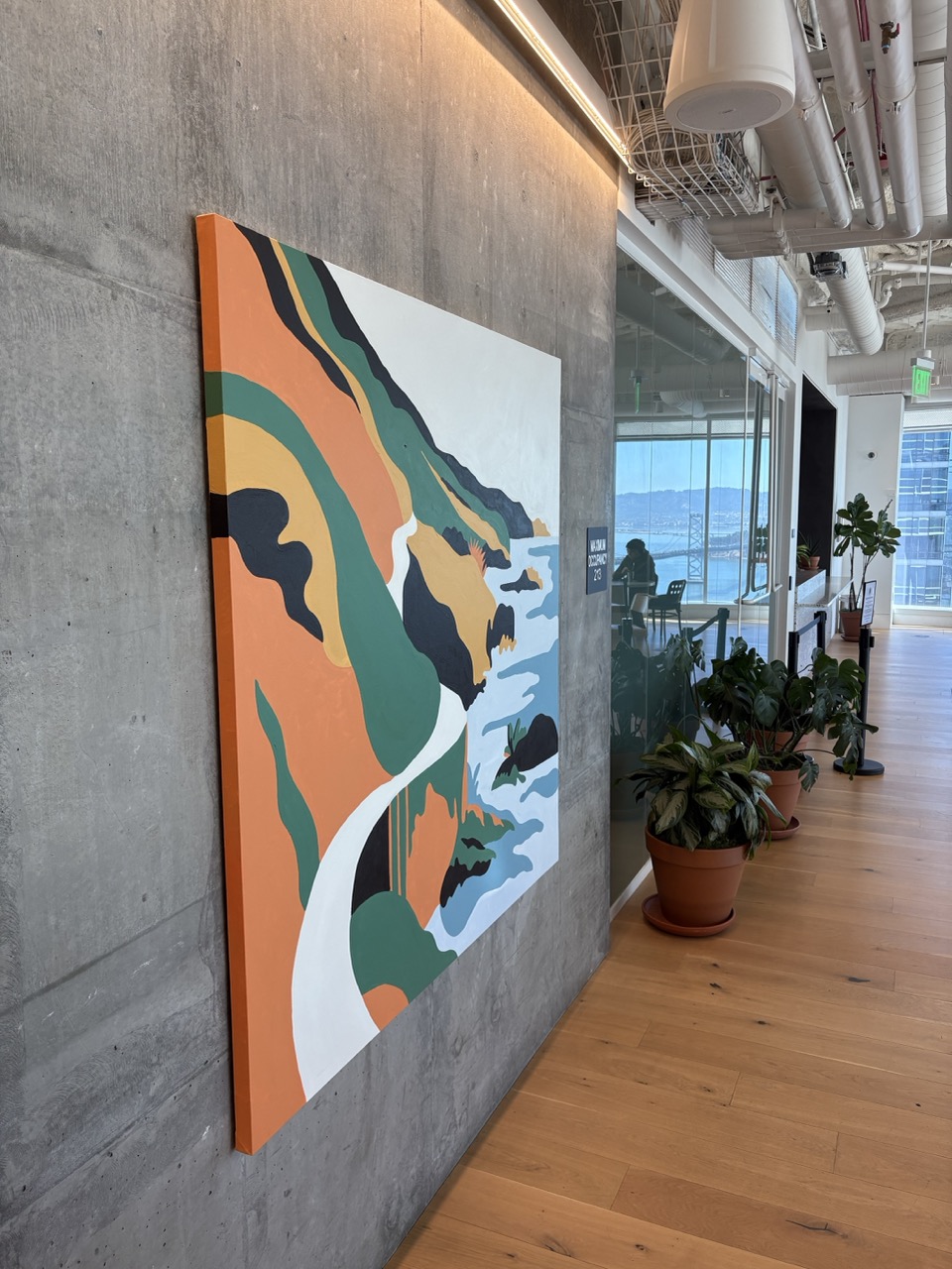
Rectification examples
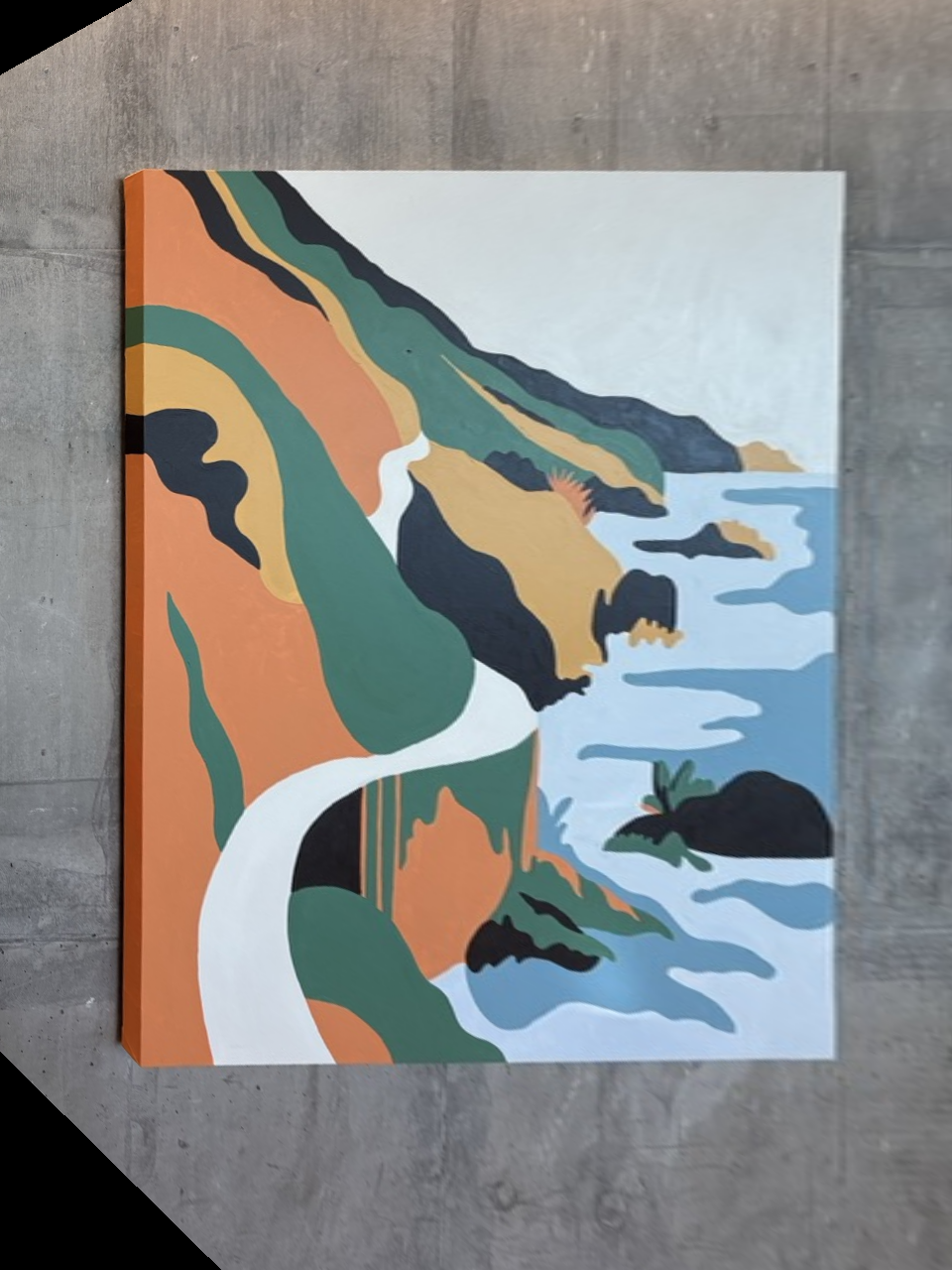
Example 1: I photographed this image from the side. By applying a homography, I rectify the planar surface and change the perspective so it appears as if viewed straight from the front.

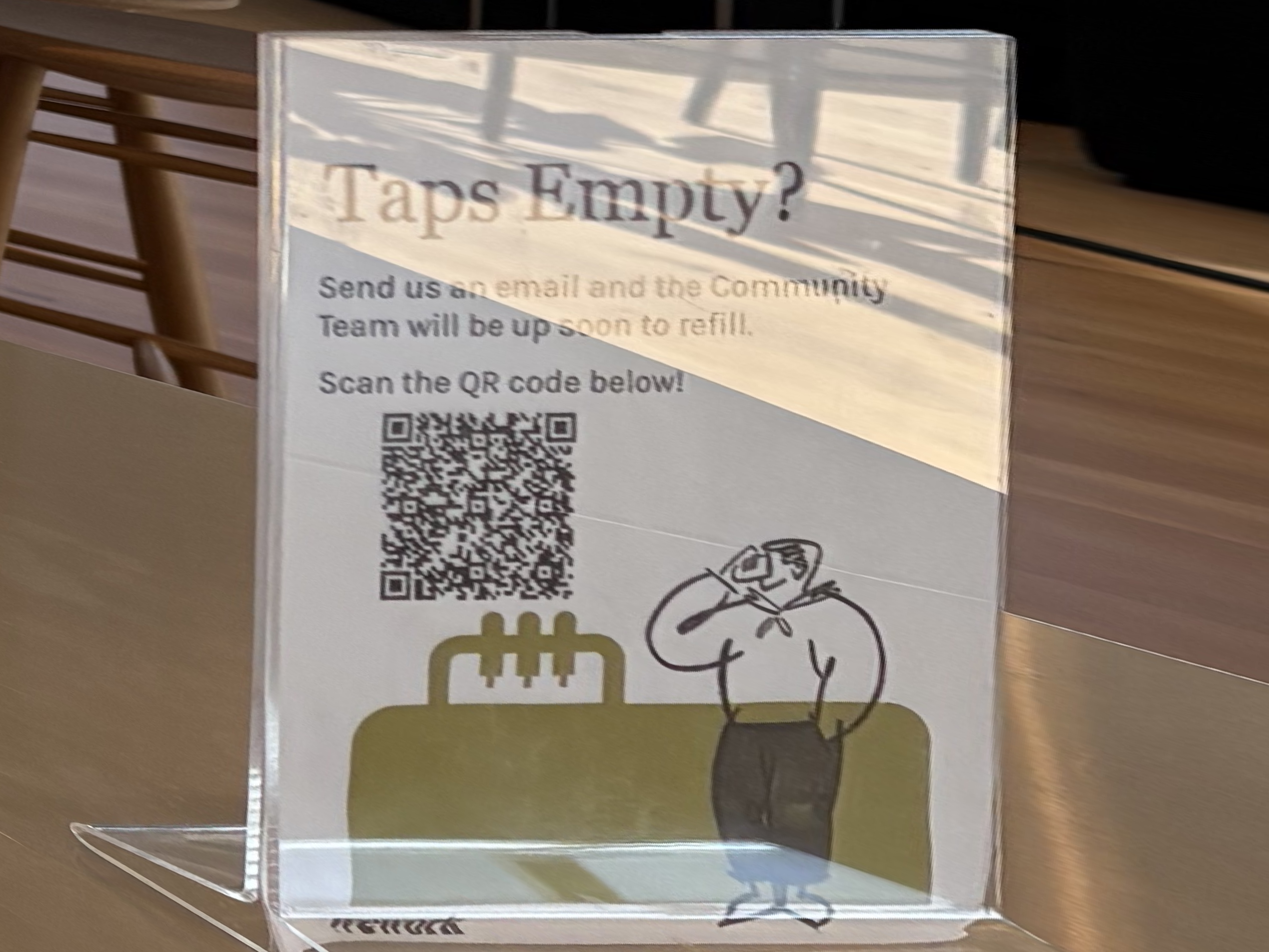
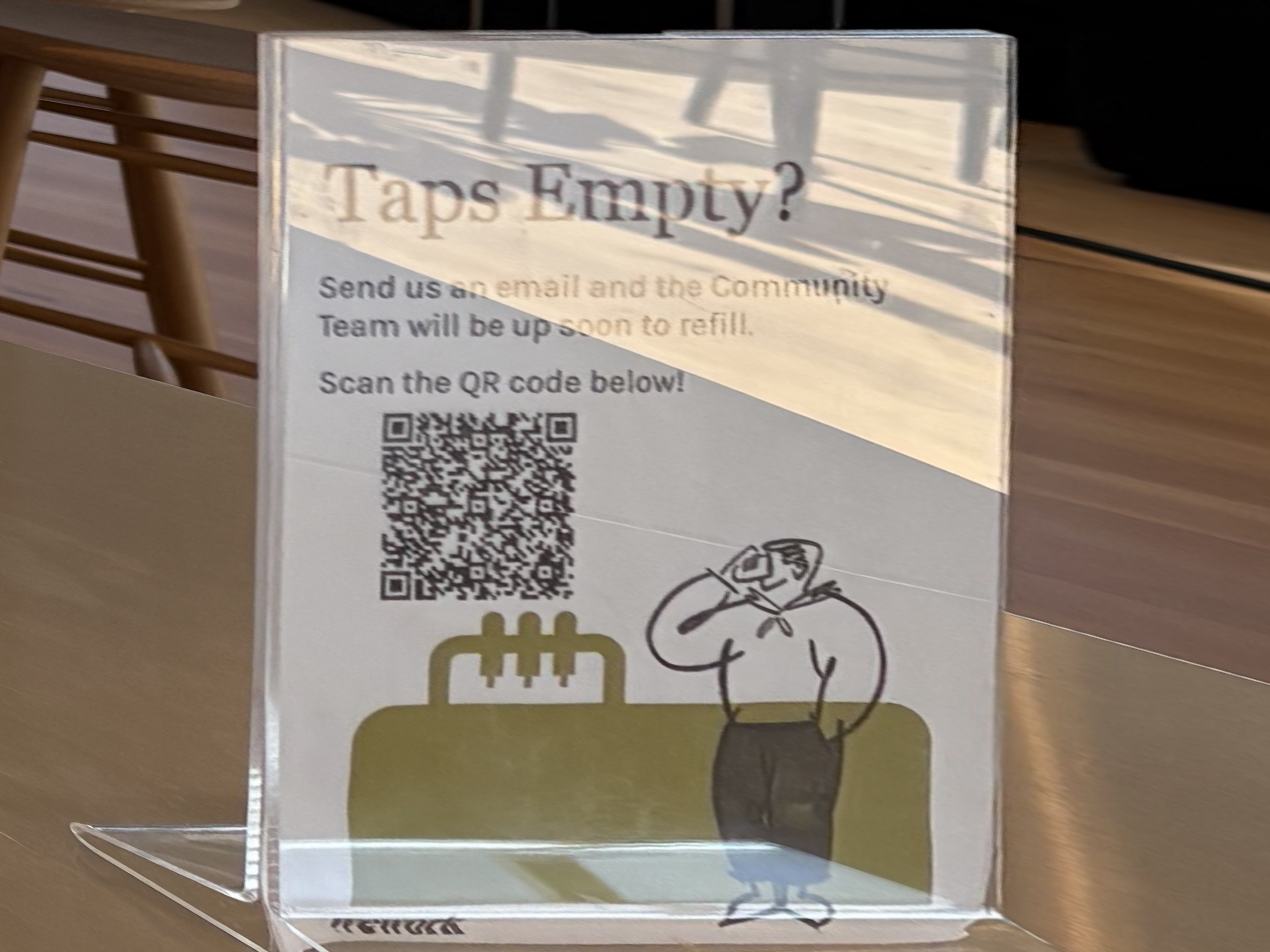
Example 2: I found a sign tilted sideways. It is hard to read like this! After applying my rectification techniqye, the sign is upright and the text is easily readable.
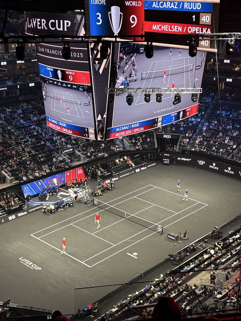
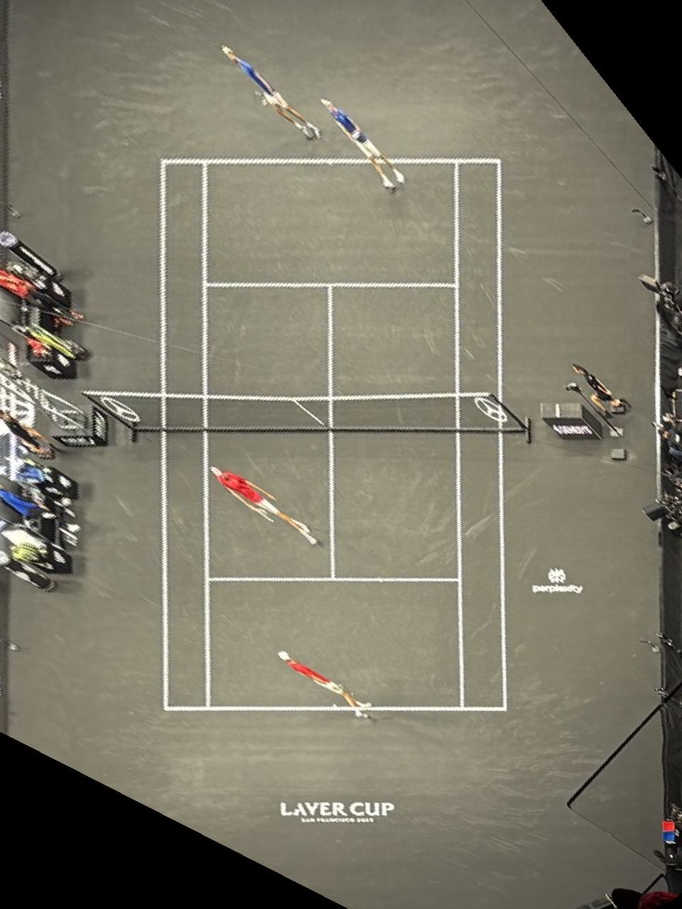
Example 3: I attended the Laver Cup tennis tournament in SF. From this steep angle it’s hard to judge if a ball was in or out. With rectification we get a bird’s‑eye view of the court — no Hawk‑Eye needed!

Warping one image into the plane of the other
Interpolation comparison
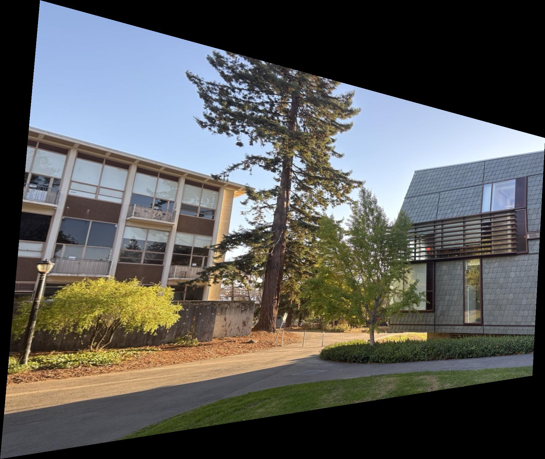
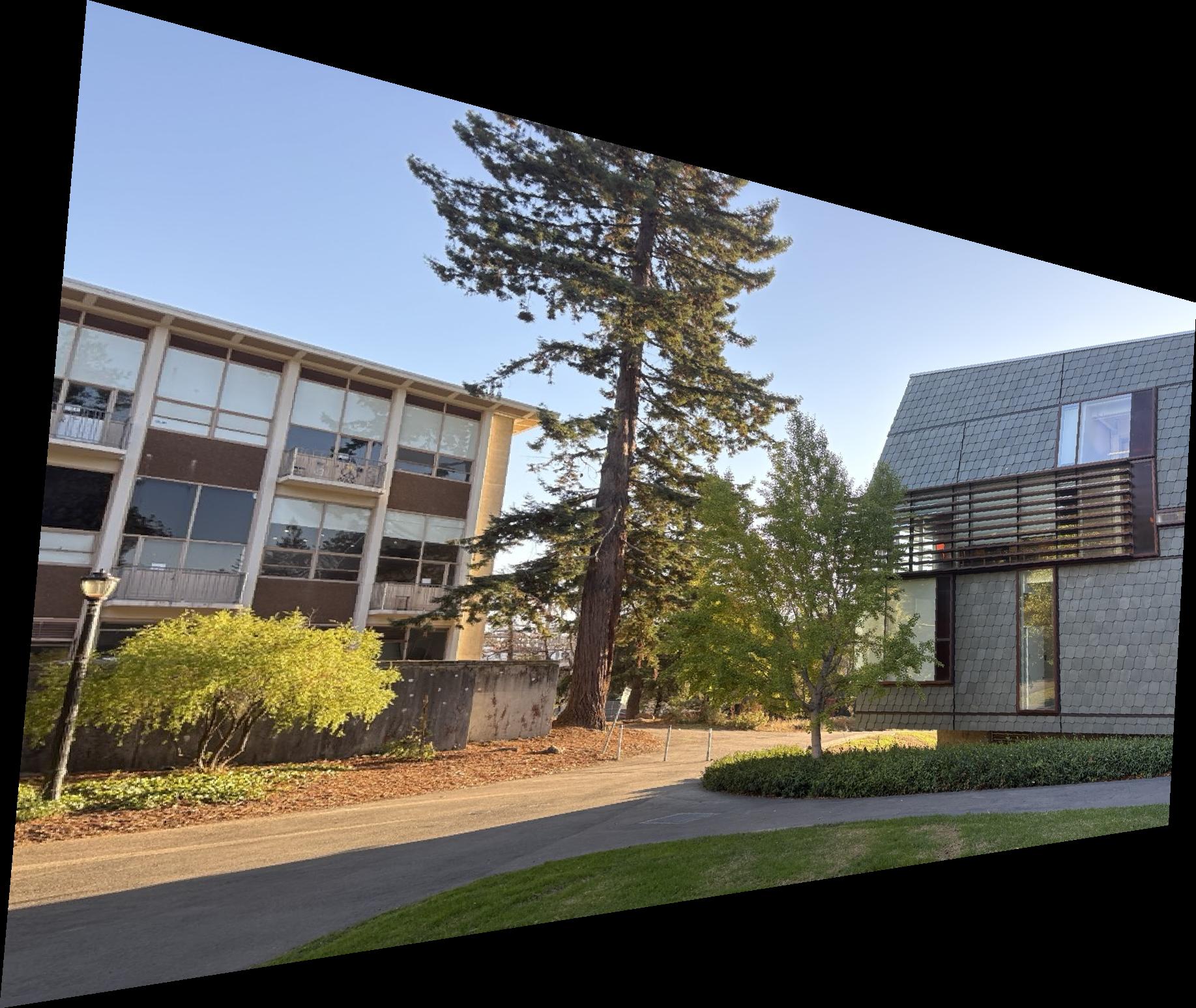
You can use the image sliders on this page to directly compare the methods—drag the handle to reveal differences. Bilinear interpolation consistently looked better in my results when comparing to nearest neighbor. When dragging the slider and inspecting the zoomed window, nearest neighbor shows blocky artifacts; straight edges—especially diagonal or slanted lines—break and look less clean. Bilinear is slightly smoother. I can appeach a bit blurrier, but it preserves line continuity and reduces aliasing, so edges and window frames look noticeably cleaner overall.
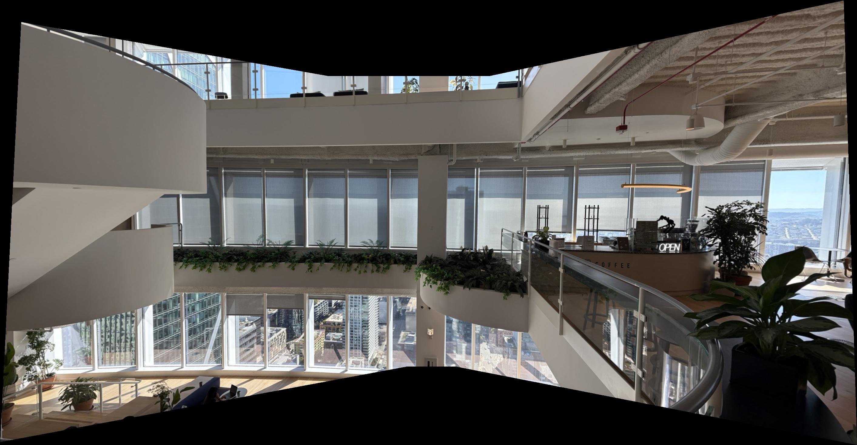
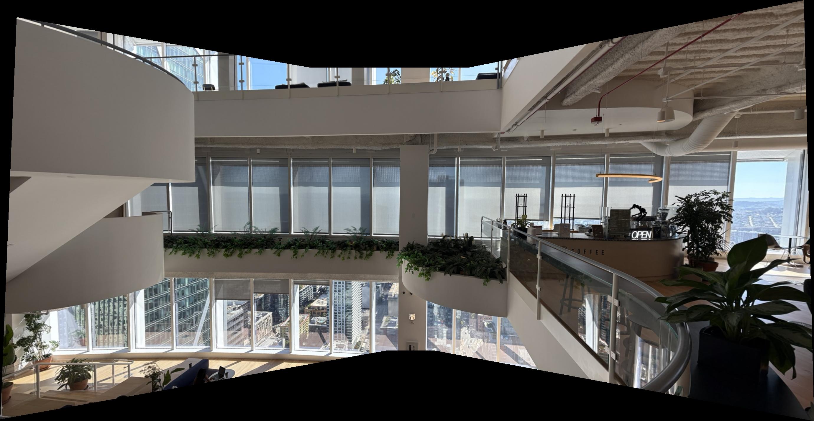
A.4: Blend Images into a Mosaic
Now I stich together the warped images into one combined mosiac.
Step 1 — Reference + inverse mapping
- Select the reference image that defines the final image plane.
- For each other image:
- Estimate its homography H to the reference image.
- Apply H to the corners to know where it lands on the final plane.
- Iterate over integer pixels inside that outline and use the inverse mapping H−1 to look up the sub‑pixel source coordinate from the to-be-warped image.
- Sample the source with bilinear interpolation (as in A.3, cleaner than nearest).
- Compute the global minima and shift all images tensors together so the composite canvas is non‑negative and starts at (0,0).
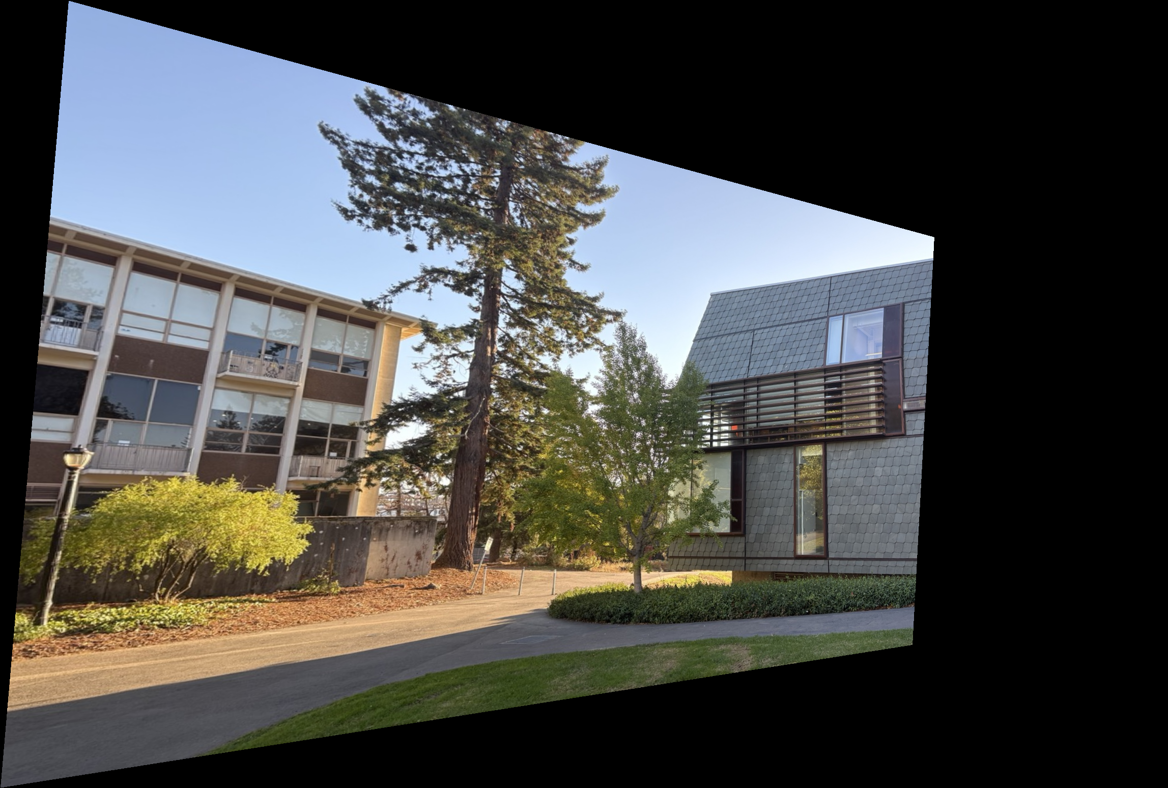
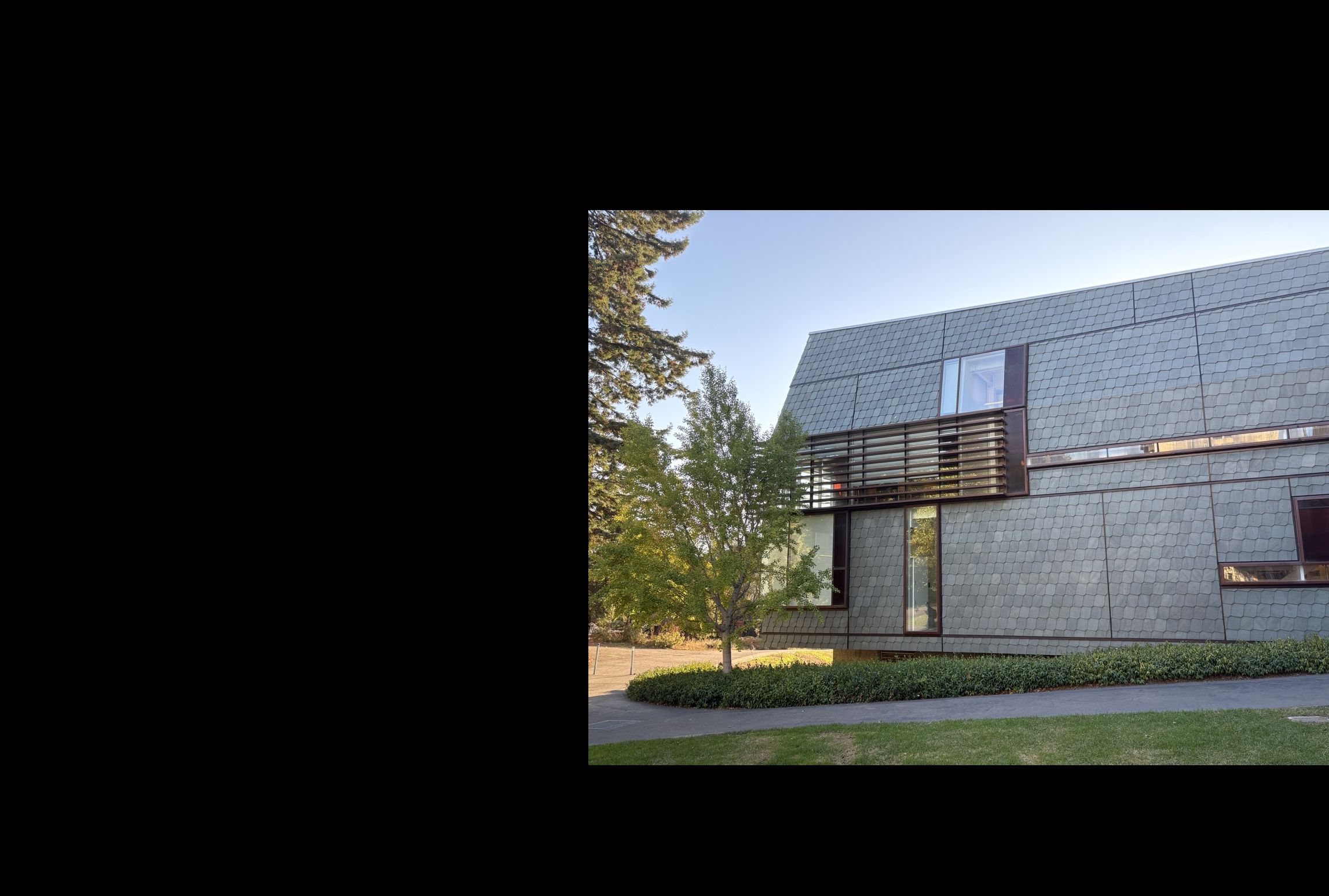
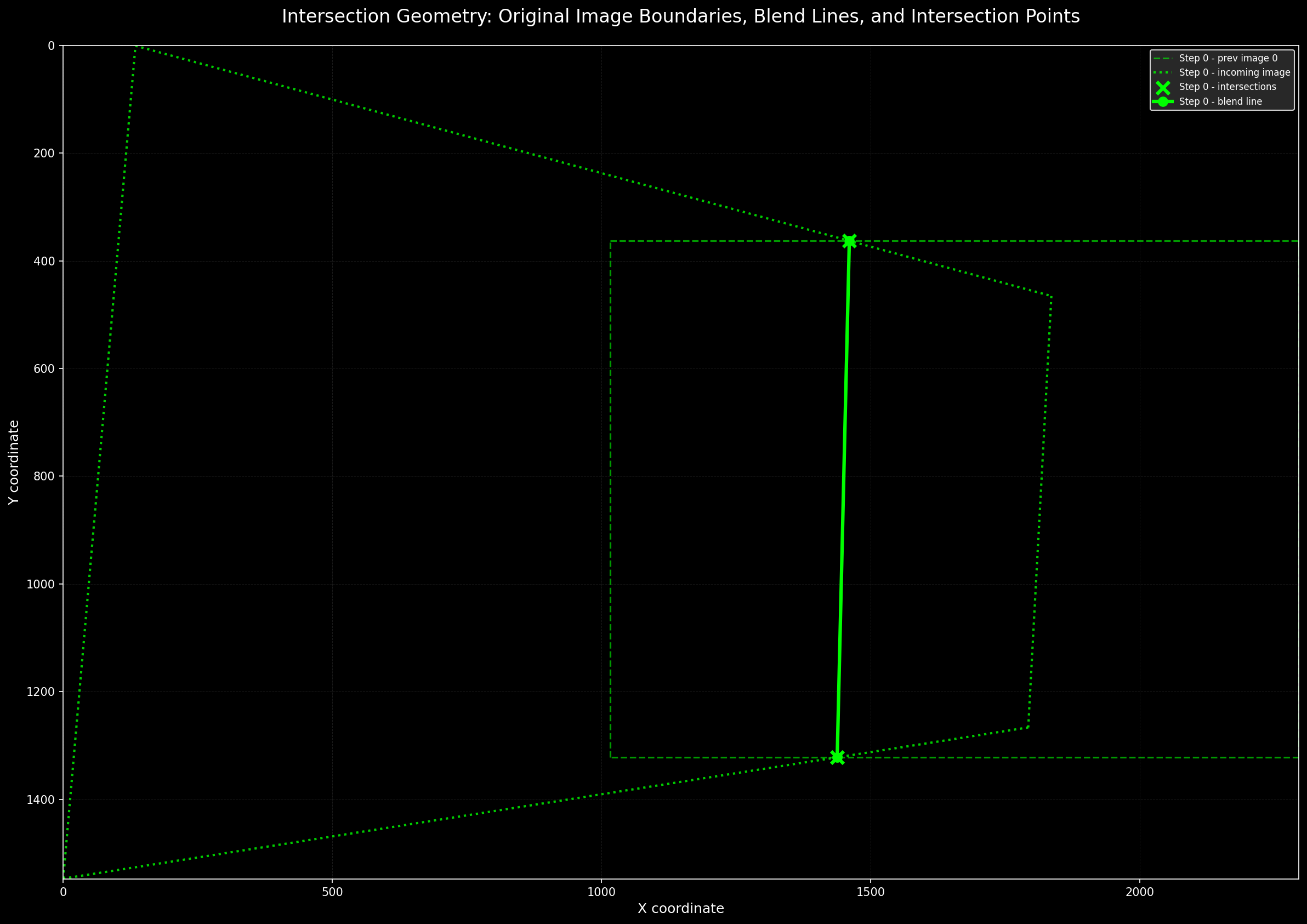
Step 2 — Seam via intersections
- For each warped image polygon, use the corners to derive line equations for each edge.
- Compute all intersections between overlapping polygons; keep the two that lie inside both shapes.
- Draw the straight line through these two points; this becomes the blend seam.
- Build a user‑specified linear blendline around the seam to create the fade masks for compositing.
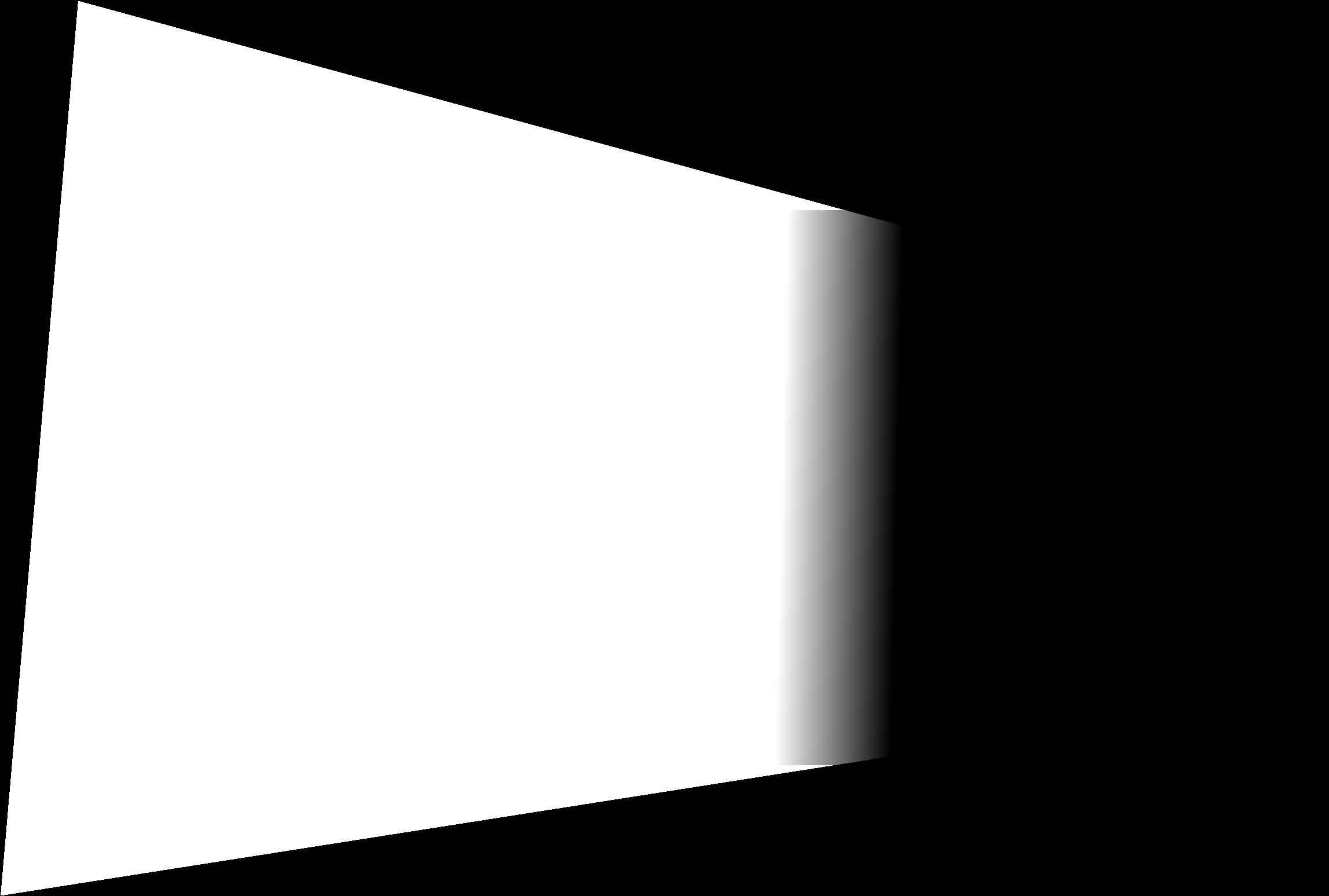
Step 3 — Composite with fade masks
- Using the fade mask, I then finally combine all image tensors into one final mosaic by multiplying each image’s pixels by its mask scale to blend contributions.

Example 2
Example 3


A.5: Bells & Whistles
Cylindrical projection: the camera rotates in place, so each image column corresponds to a viewing direction rather than a position. I map the image on a virtual cylinder wrapped around the camera and then “unroll” that cylinder to a flat canvas. Intuitively, the horizontal axis becomes the angle which the camera turned (so that theseams align naturally), while the vertical axis is slightly adjusted to avoid stretching. Using the focal length to convert pixels to angles (e.g., \(\theta = (x-\,c_x)/f\)) keeps vertical lines upright and removes the strong perspective squeeze that would otherwise appear at the edges of my panorama.
Formulas I used (principal point \((c_x,c_y)\), focal length \(f\)):
Unroll plane → cylinder (compute cylinder coords \((u,v)\) from image pixel \((x,y)\)):
\[
\theta = \arctan\!\Big(\frac{x - c_x}{f}\Big),\quad
u = c_x + f\,\theta,\quad
v = c_y + \frac{y - c_y}{\cos\theta}.
\]
Sample back cylinder → plane (map canvas \((u,v)\) to source \((x,y)\) for bilinear lookup):
\[
\theta = \frac{u - c_x}{f},\quad
x = c_x + f\,\tan\theta,\quad
y = c_y + (v - c_y)\,\cos\theta.
\]
This reparameterization makes yaw rotations look more like horizontal shifts on the cylinder. It thereby reduces perspective squeeze at wide fields of view while preserving verticals. I then align the warped views on a common canvas and blend overlaps with the same technique as in the previous section.
B.1: Harris Corner Detection and ANMS
Here, as advised, I foolow the approach from “Multi‑Image Matching using Multi‑Scale Oriented Patches”. he pipeline begins with Harris interest points before selection by ANMS.
Harris detects points where intensity changes strongly in two orthogonal directions. Using image gradients \(I_x, I_y\) and a Gaussian window \(G_\sigma\), we build the second‑moment matrix
\[
M = G_\sigma * \begin{bmatrix} I_x^2 & I_x I_y \\ I_x I_y & I_y^2 \end{bmatrix}.
\]
The Harris response scores corners as shown in the equation below.
\[
R = \det(M) - k\,\mathrm{tr}(M)^2,\quad k \in [0.04, 0.06].
\]
Only points whose the Harris response was strictly greater than all neighbors were used and are visible in the Figure below.
Note: I used the provided
harris.py script for the Harris corner detection step; it handled the first part.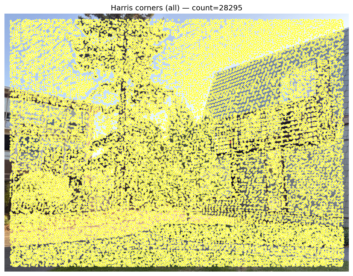
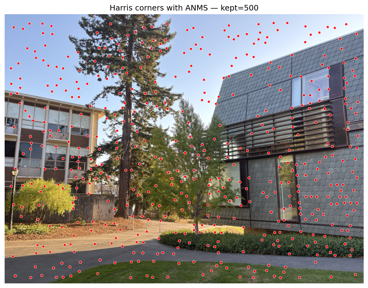
Adaptive Non‑Maximal Suppression (ANMS)
Harris responses are pruned with ANMS to obtain spatially uniform and high‑quality keypoints. We assign each candidate a suppression radius using its strength \(f(\mathbf{x})\): \[ r_i = \min_j \; \|\,\mathbf{x}_i - \mathbf{x}_j\,\| \quad \text{s.t.}\quad f(\mathbf{x}_i) < c_{\text{robust}}\, f(\mathbf{x}_j),\; \mathbf{x}_j \in \mathcal{I}. \] I use \(c_{\text{robust}} \approx 0.9\). Points with no stronger neighbor receive a large sentinel radius (e.g., image diagonal). Finally, I select the top‑K largest radii (K≈500) as the keypoints from ANMS.B.2: Feature Descriptor Extraction
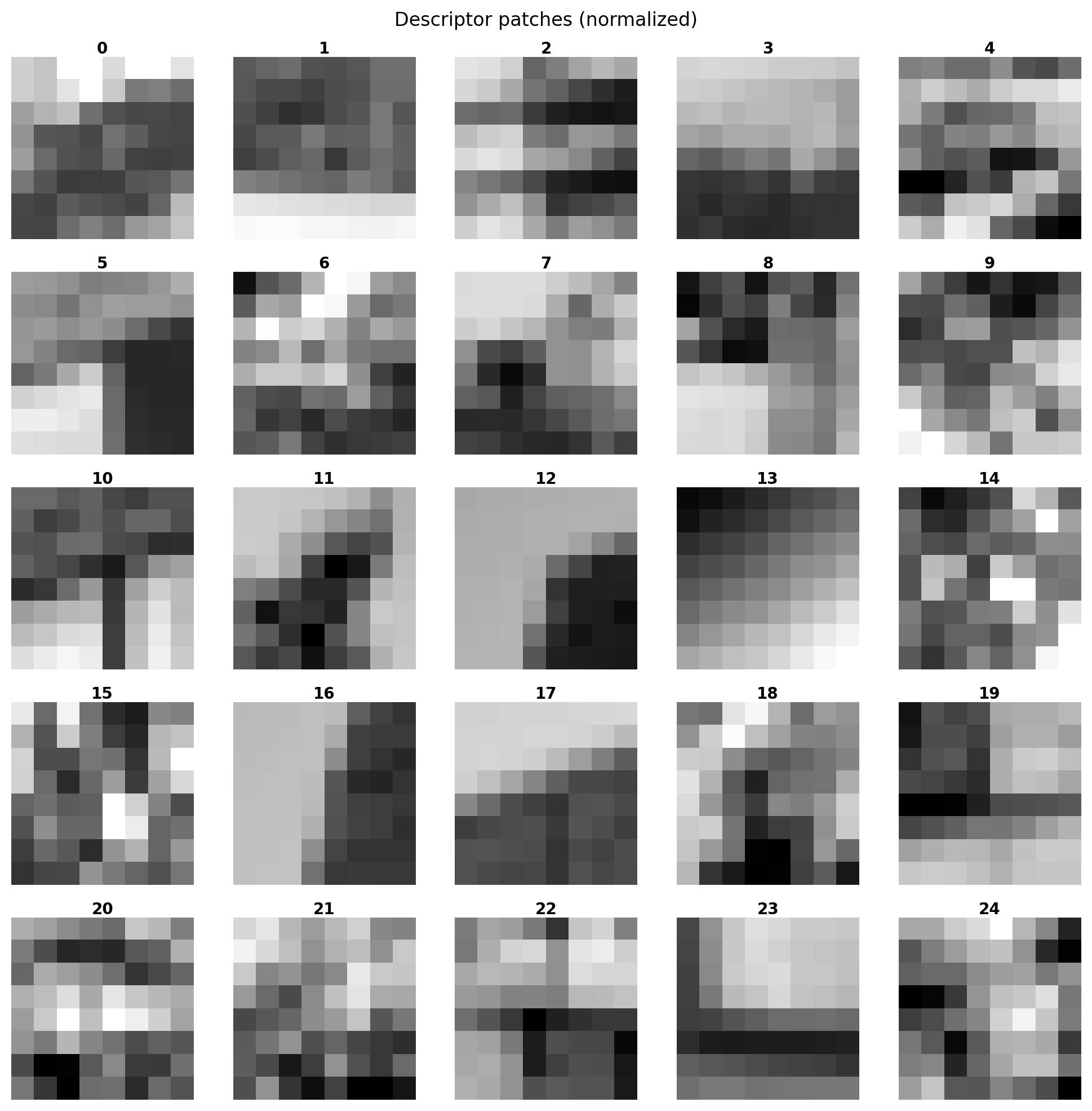
Next, I follow MOPS approach: sample a normalized intensity patch around each ANMS keypoint. The original work proposes multi‑scale oriented patches; here I adopt the same spirit with a single‑scale variant (and later in the Bells & Whisltes also implement a multi‑scale variant)
- Use the top‑K keypoints from B.1 (Harris + ANMS; K≈500).
- Theextract a 40×40 patch around each keypoint.
- Resample each cntext window bilinear from 40×40 to 8×8.
- Flatten to 64‑D and apply bias/gain normalization \((v - \mu)/\sigma\) to reduce lighting effects, as advocated by the paper.

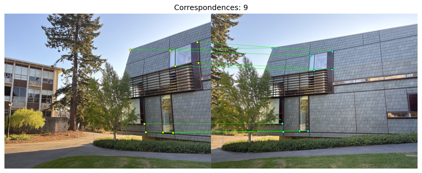
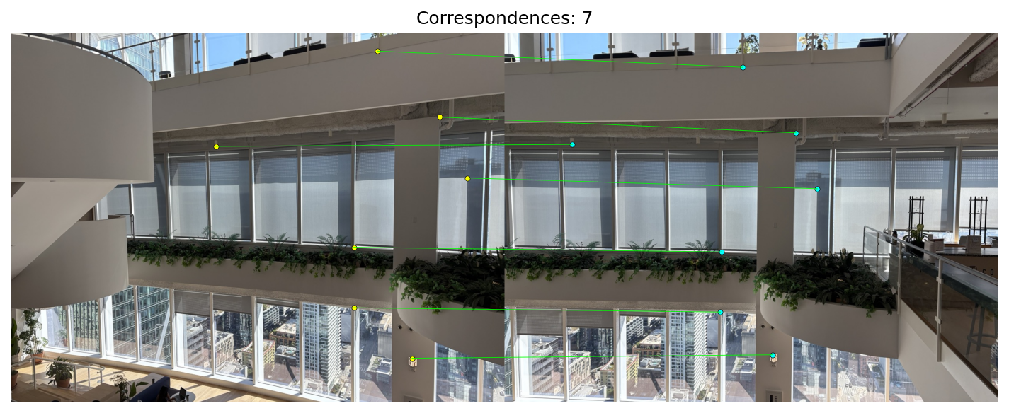
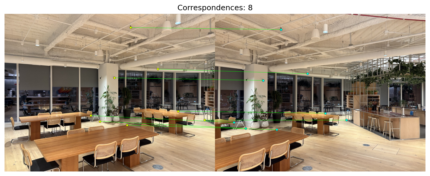
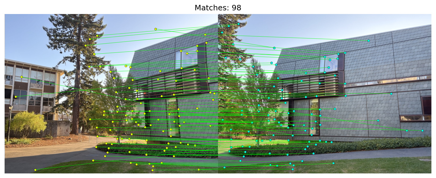
B.3: Feature Matching
Following the matching strategy common to MOPS/SIFT pipelines, I compare descriptors with squared Euclidean distance and apply Lowe's ratio test.
Given two descriptor sets \(\{\mathbf{d}_i\}_{i=1}^{N_1}\) and \(\{\mathbf{d}'_j\}_{j=1}^{N_2}\), I compute the full distance matrix efficiently via
\[
D_{ij} = \|\mathbf{d}_i - \mathbf{d}'_j\|_2^2 = \|\mathbf{d}_i\|_2^2 + \|\mathbf{d}'_j\|_2^2 - 2\, \mathbf{d}_i^\top \mathbf{d}'_j.
\]
I build a full distance matrix: each row corresponds to one feature in image 1, and each column to one feature in image 2. Entry \(D_{ij}\) is the distance from feature i to feature j in the other image.
For each \(i\), let \(d_1\) and \(d_2\) be the smallest and second‑smallest distances in row \(i\) (best and runner‑up). The ratio test keeps a match only if
\[
r_i = \frac{d_1}{d_2} < \tau, \quad \text{with } \tau\approx 0.65.
\]
Ref: Figure 6b in Brown–Szeliski–Winder suggests ~0.65 as a sweet spot: above this, incorrect matches dominate; below this, correct matches dominate.
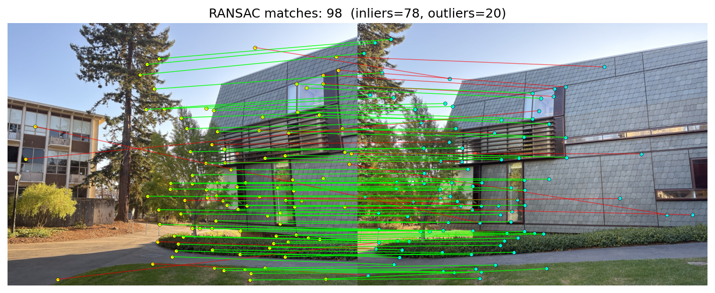
B.4: RANSAC for Robust Homography
Given tentative matches from B.3, I estimate a projective homography with RANSAC.
In homogeneous coordinates, corresponding points satisfy
\[
\tilde{\mathbf{x}}_2 \;\sim\; H\,\tilde{\mathbf{x}}_1,\qquad \tilde{\mathbf{x}} = [x\;y\;1]^\top,\; H \in \mathbb{R}^{3\times 3}.
\]
After dehomogenization (divide by the third component), I score using the symmetric transfer error
\[
E_i = \big\|\mathbf{x}_2^{(i)} - \pi(H\,\tilde{\mathbf{x}}_1^{(i)})\big\|_2^2\; +\; \big\|\mathbf{x}_1^{(i)} - \pi(H^{-1}\,\tilde{\mathbf{x}}_2^{(i)})\big\|_2^2,
\]
where \(\pi([X\;Y\;Z]^\top) = [X/Z\;Y/Z]^\top\). A correspondence is an inlier if \(E_i < \tau^2\) (here \(\tau\approx 3\) px).
The algorithm:
- Sample 4 matches uniformly; compute a candidate \(H\) from the minimal set.
- Score by counting inliers under the symmetric transfer error threshold.
- Keep the best model (max inliers) over T iterations.
- Refit \(H\) using all inliers from the best model for the final estimate.
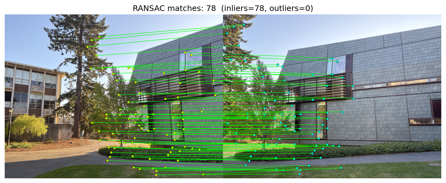
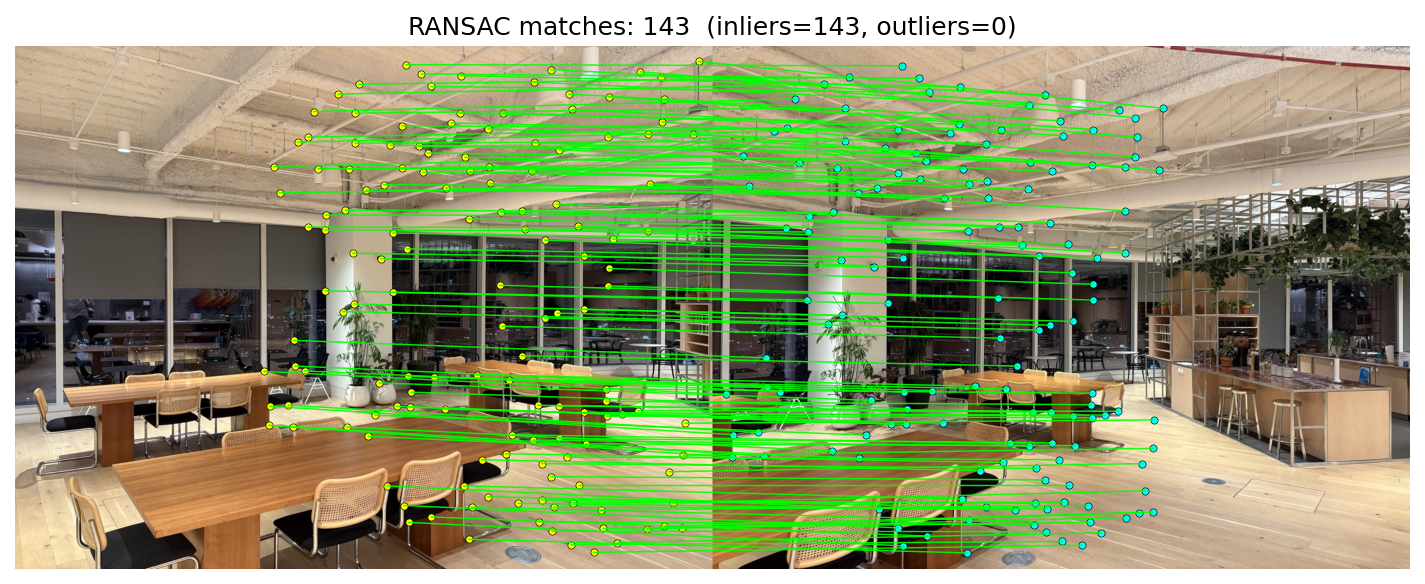
Manual vs RANSAC mosaics
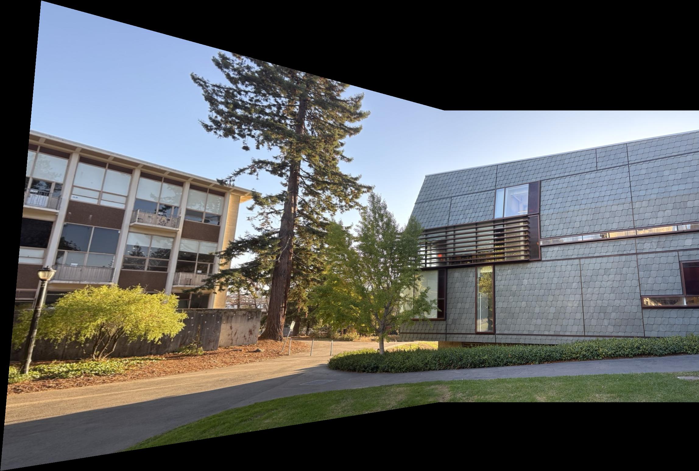
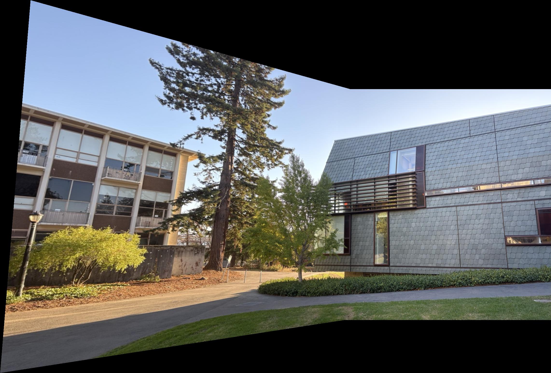


Overall, the RANSAC‑based approach outperformed my manual correspondence picks. If you closely inspect the blending regions—for example, in Set 3 near the bottom middle where all three images intersect—the manual mosaic looks noticeably blurrier, whereas the RANSAC result remains clean and well‑aligned.
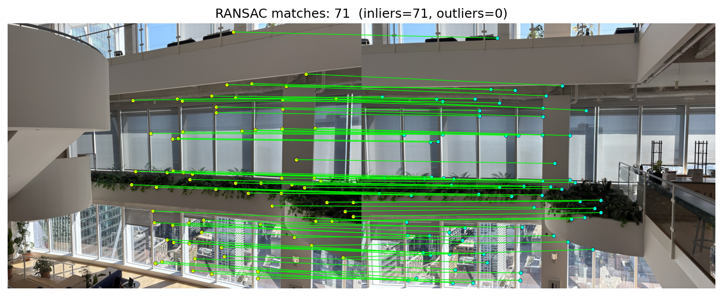
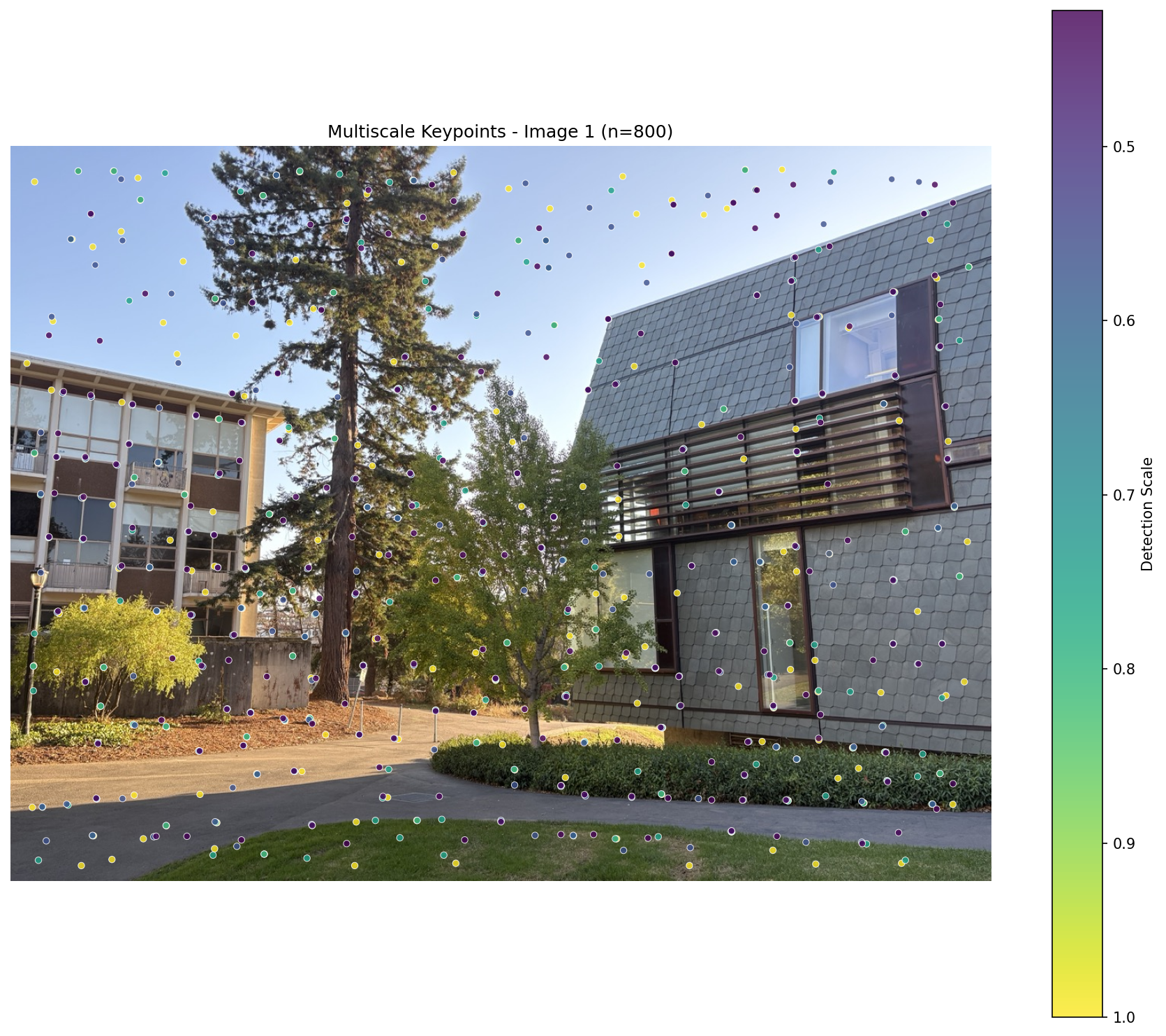
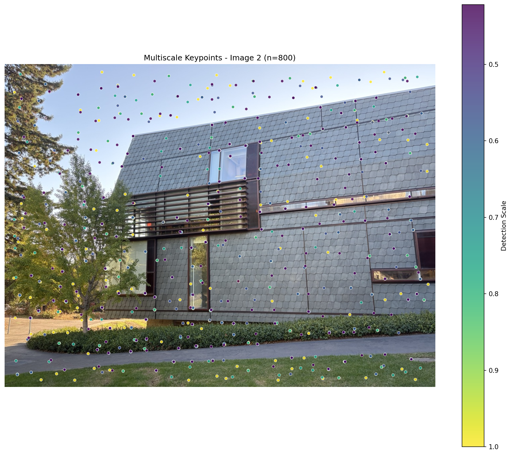
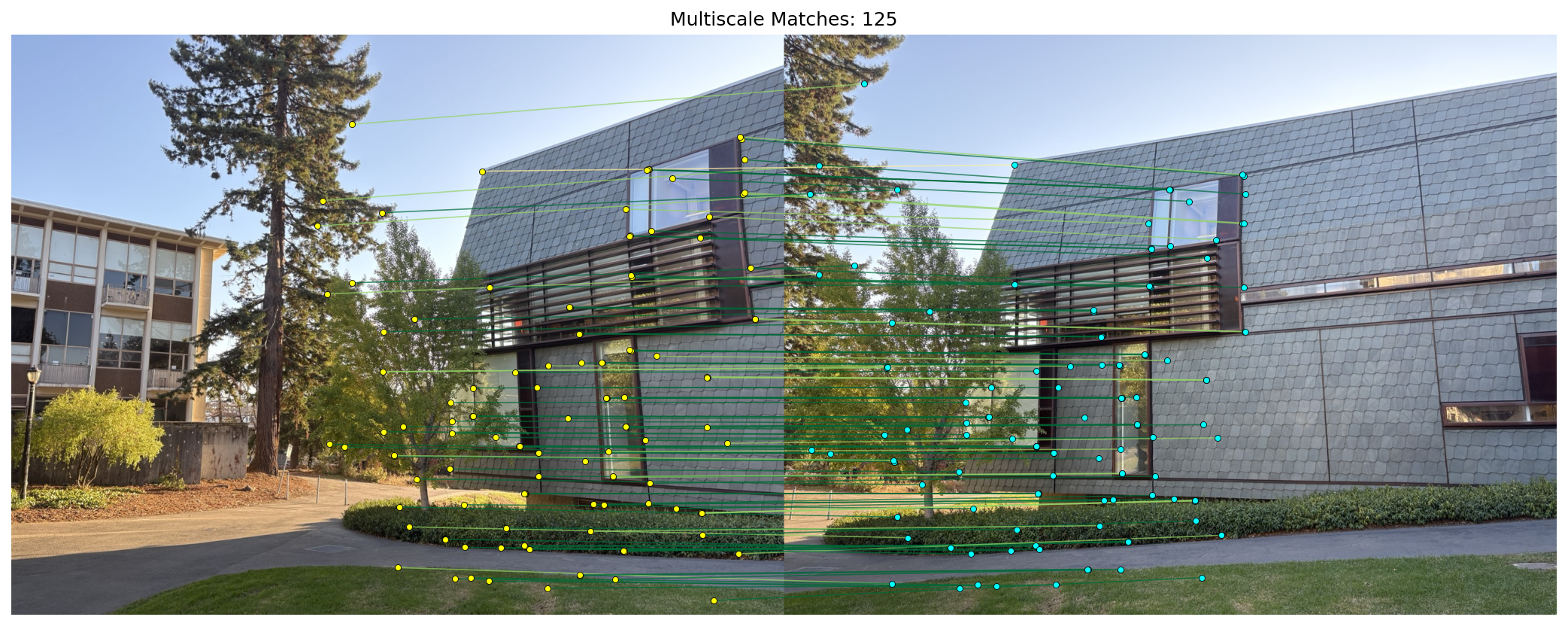
B.5: Multiscale Feature Detection and Matching
Building on B.1–B.4, I make the pipeline scale‑aware with a pyramid: at each level I run Harris (B.1) → ANMS (B.1) → MOPS‑style 8×8 descriptors (B.2), then match with Lowe’s ratio and optional mutual check (B.3). I estimate a homography with RANSAC (B.4) and show all matches vs. inliers.
How the pyramid works (simple):
- Start from the original grayscale image; repeatedly downscale by a factor (f.e. 0.75).
- At each level, run Harris + ANMS and extract 40×40 → 8×8 normalized patches.
- Convert keypoints to original coordinates by dividing by the level’s scale and record the detection scale.
- Concatenate features from all levels, perform matching once, then run RANSAC.
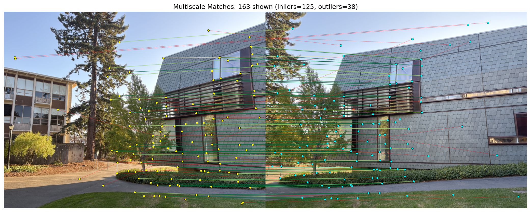
Final mosaic using multiscale features + RANSAC — it looks very lean with the multiscale approach.
