Project 4
CS180/280A: Intro to Computer Vision and Computational Photography
Neural Radiance Field!
Part 0: Calibrating Your Camera and Capturing a 3D Scan
Part 0.1: Calibrating Your Camera
- Captured 53 calibration images at a fixed zoom.
- Detected ArUco corners and computed intrinsics/distortion via
cv2.calibrateCamera. - Skipped frames without detections to avoid corrupting calibration.
- Used ProCam to lock exposure, white balance, shutter speed, and ISO; kept autofocus enabled for reliable tag detection.
- My printer could not print true-to-scale, so I remeasured the printed sheet and used these dimensions in calibration: ArUco tag length 53.5 mm, horizontal separation 27 mm, vertical separation 14 mm.
Calibration image samples
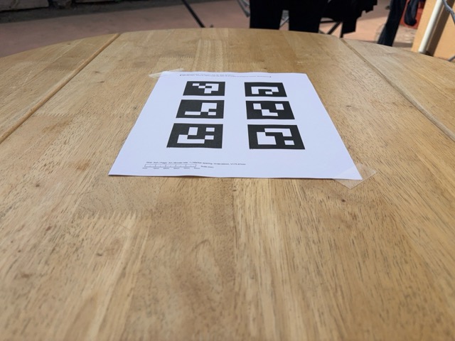
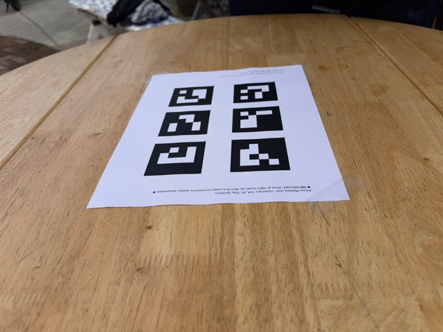
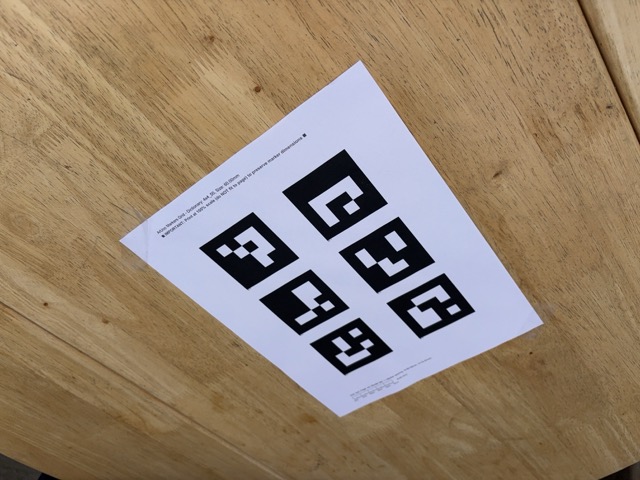
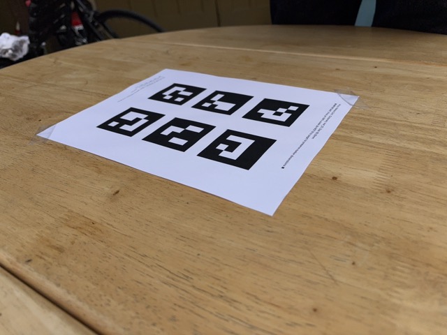
Four example frames used for camera calibration.
Part 0.2: Capturing a 3D Object Scan
- Captured 59 object images next to a printed ArUco tag.
- Used the same ProCam setup to lock exposure, white balance, shutter, and ISO; left autofocus on for robust tag detection and minimized motion blur.
- For the single reference tag used during capture, the measured side length was 95.5 mm.
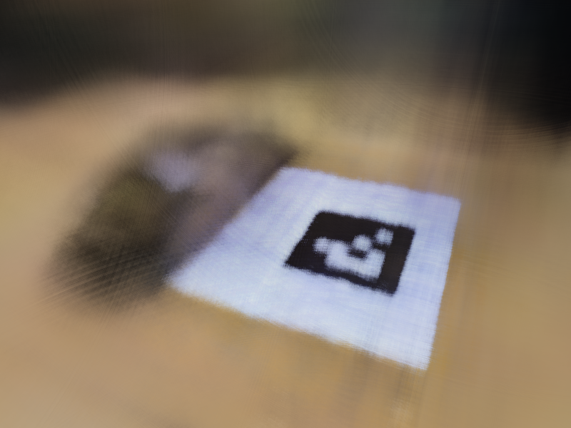
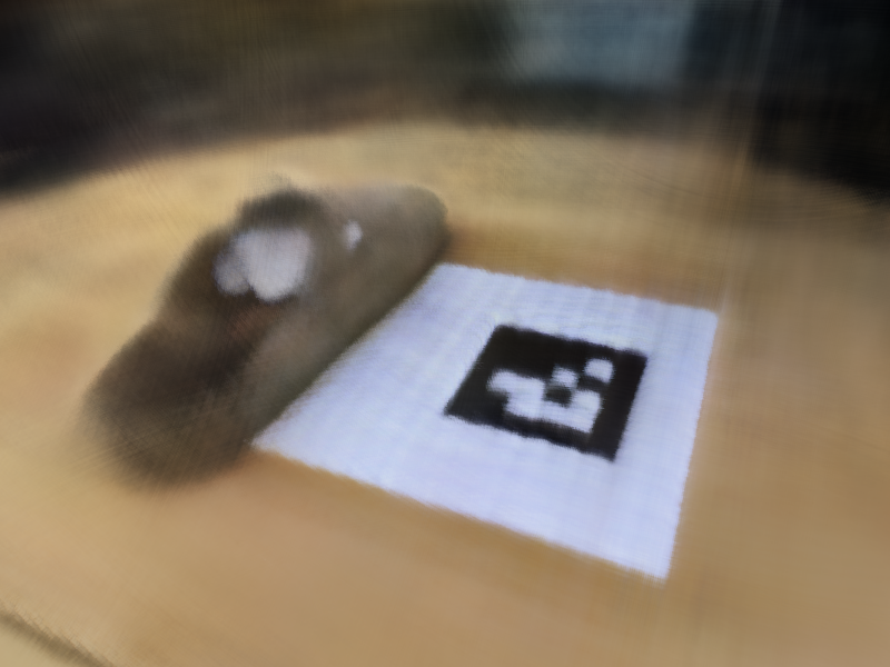
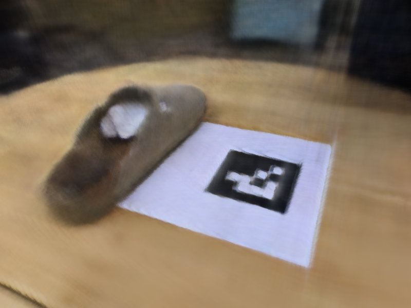
Object scan samples
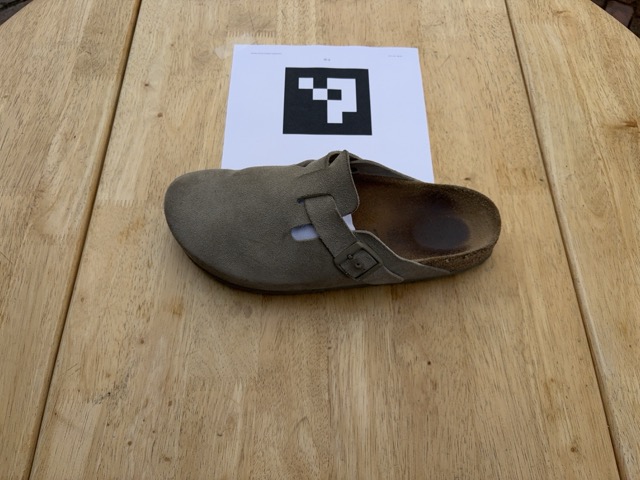
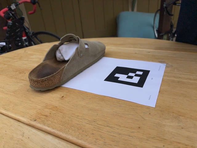
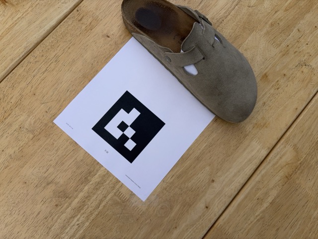
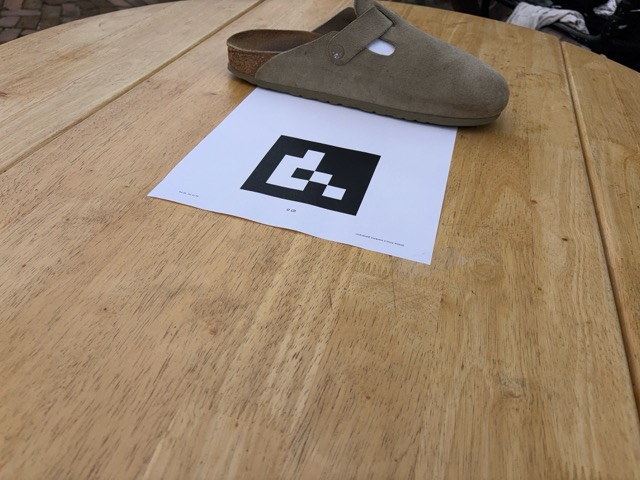
Example frames from the object capture session.
Part 0.3 + 0.4: Estimating Camera Pose and Dataset
- Used
cv2.solvePnPwith detected corners and intrinsics to recover pose. - Converted to camera-to-world matrices for visualization and later parts.
- Visualized camera frustums in 3D in Viser.
- Undistorted images with
cv2.undistort(later, I skipped the undistort step, as this yielded better results). - Using recovered intrinsics and poses (
c2w), I packaged everything into a final.npzdataset for training.
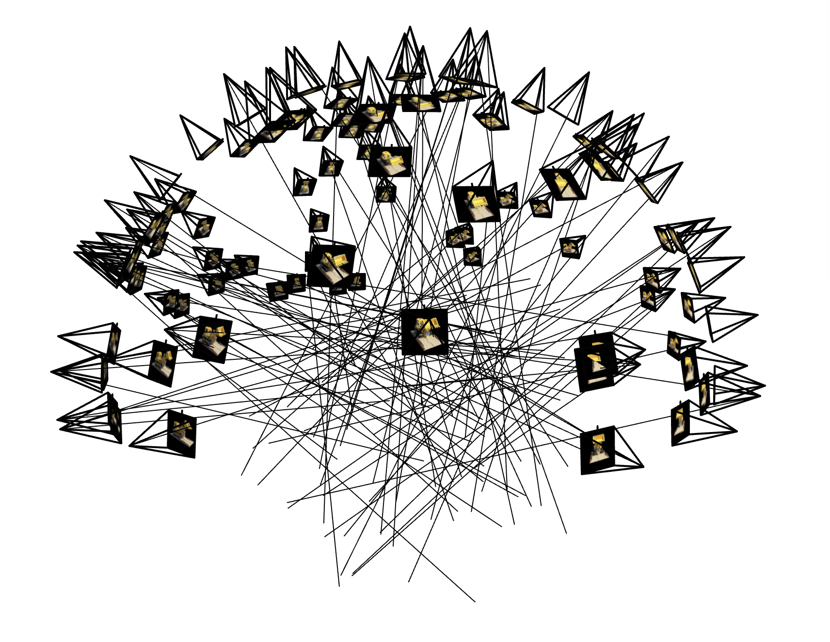
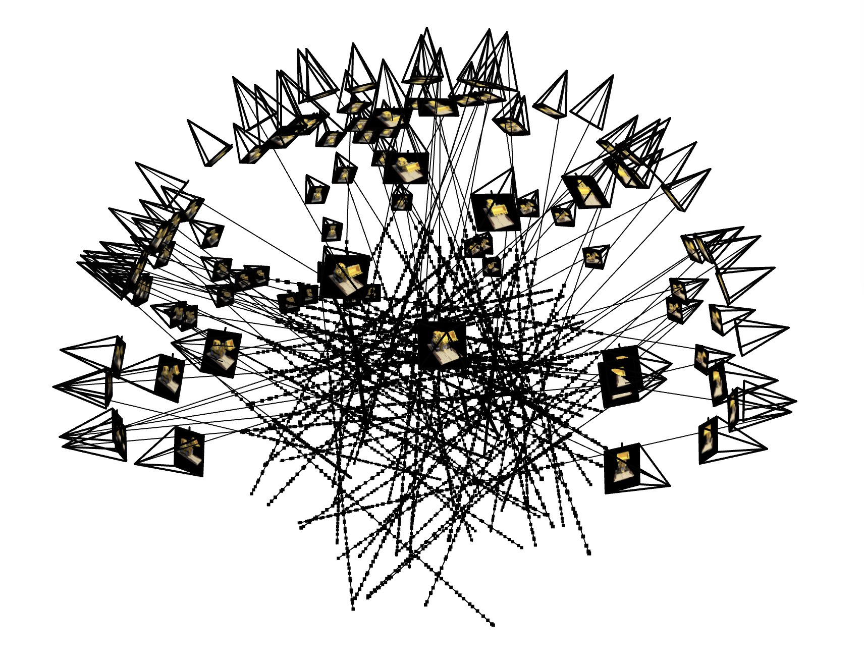
3D Visualization: Cameras, Rays, and Samples
In the visualization below, the camera-to-world (c2w) frames make it clear where each
photograph was taken from. The camera centers trace an approximately hemispherical path around the
object—covering different azimuths and elevations—so you can see angles and positions spanning a
broad arc. This is visible in the Viser plot and provides good angular coverage while keeping the
object at a roughly constant distance.
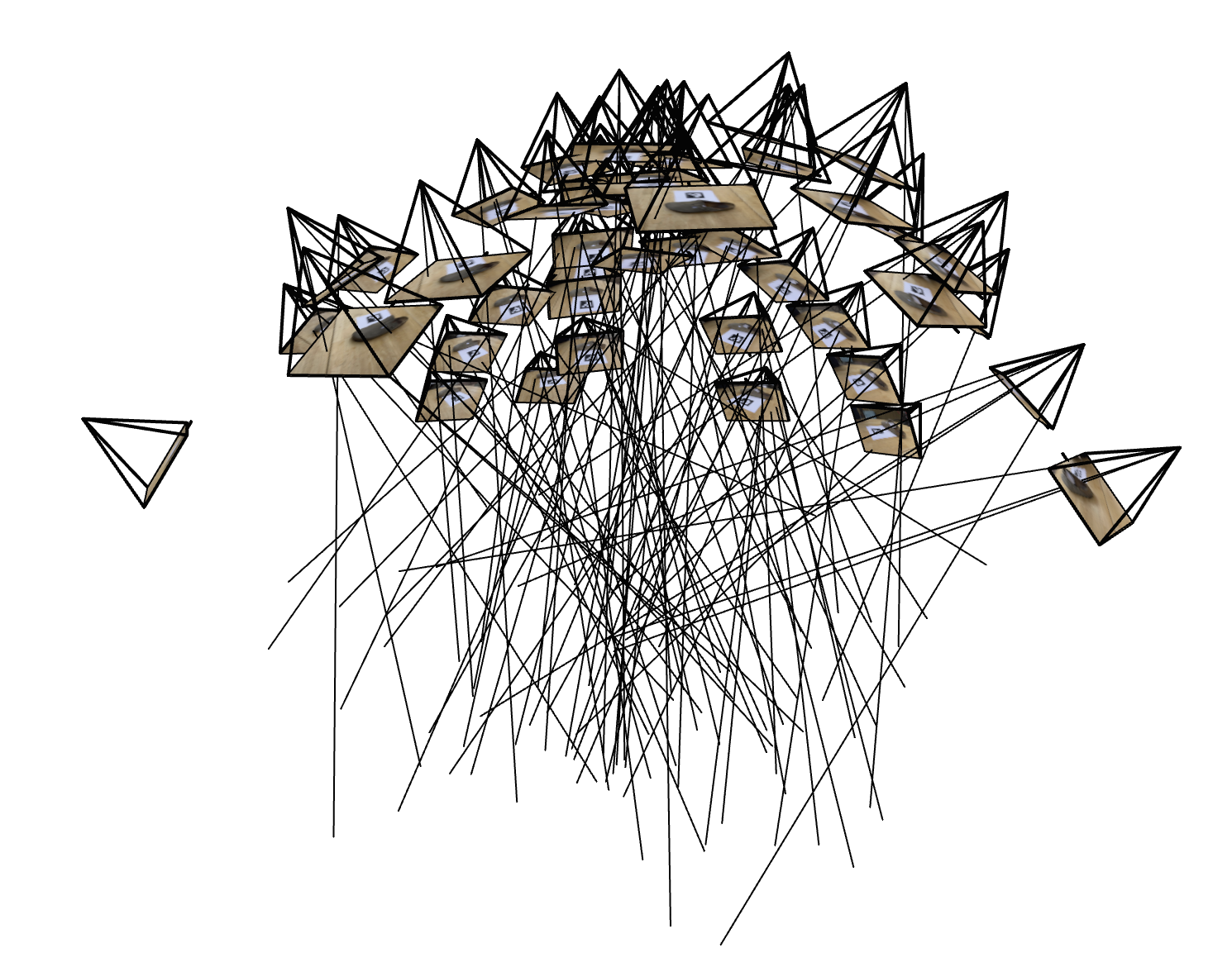
Camera frustums and sampled rays
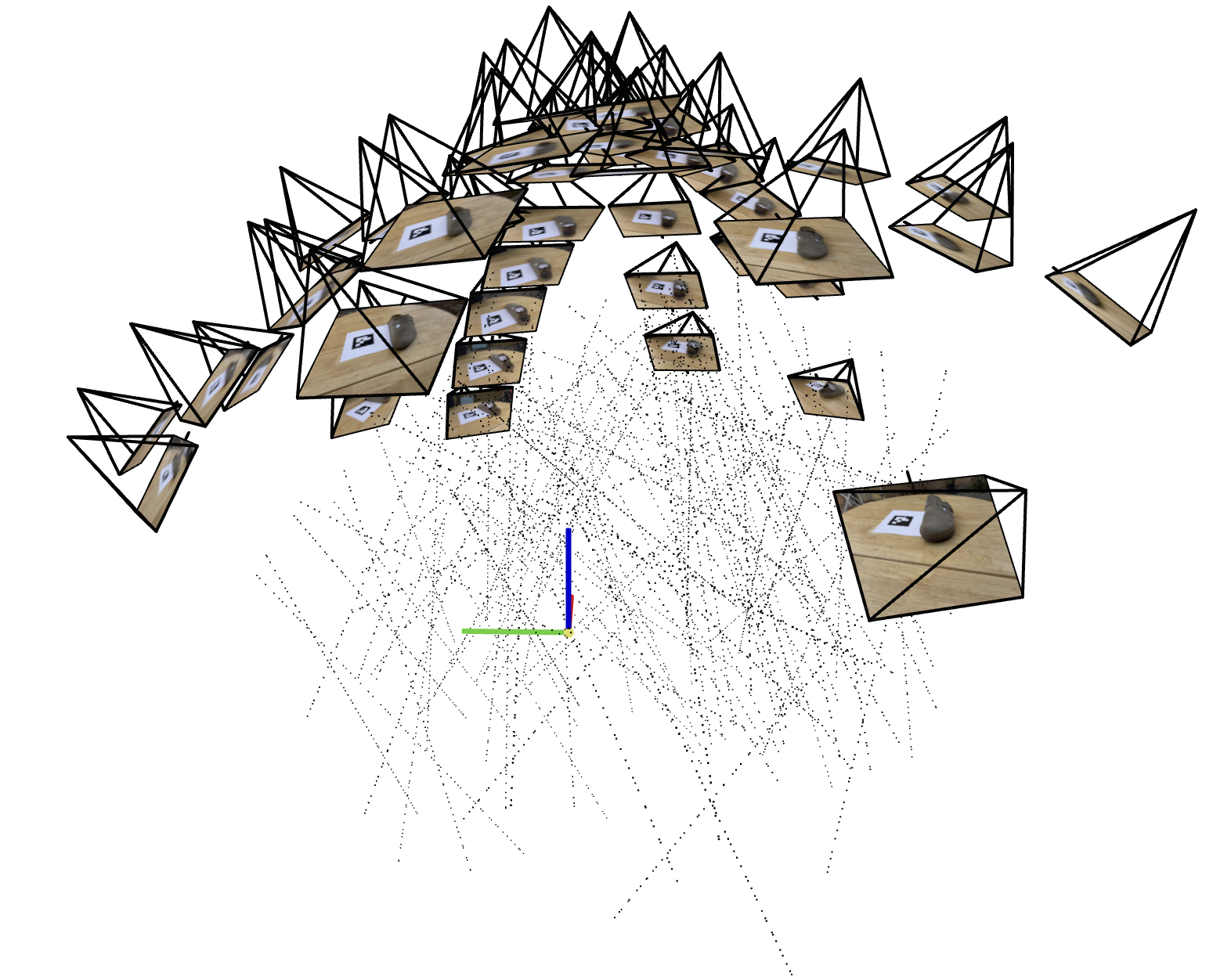
Sample points along rays for NeRF training. Origin visible at ArUco tag corner.
Part 1: Fit a Neural Field to a 2D Image
In this part, I train a neural field (an MLP with sinusoidal positional encoding) to map 2D pixel coordinates to RGB, fitting an image by minimizing mean squared error. The output quality is measured with Peak Signal-to-Noise Ratio (PSNR), which increases as MSE decreases:
Model Architecture
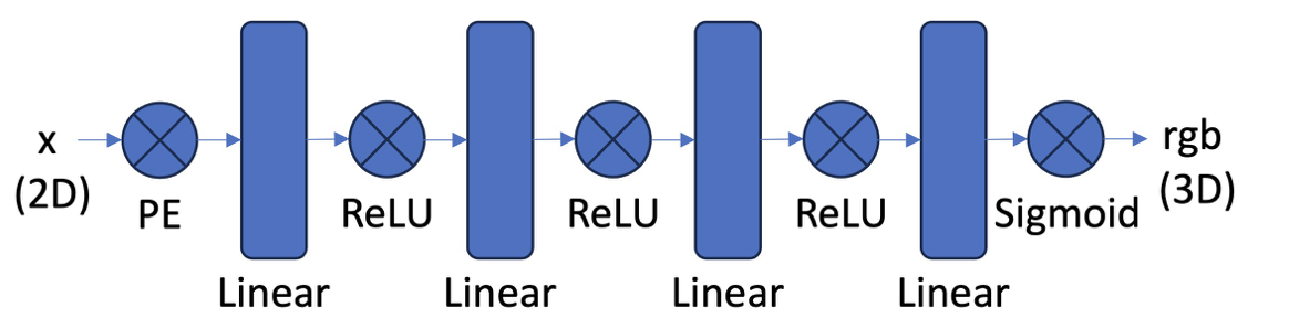
MLP with positional encoding and a skip connection.
- Implemented an MLP with sinusoidal positional encoding to map 2D coords → RGB in PyTorch.
- Used a random pixel sampling dataloader; trained with MSE (Adam 1e-2).
- Reported PSNR and tuned width and max PE frequency.
Hyperparameters (Example + Yosemite training)
| Parameter | Value |
|---|---|
| iters | 2000 |
| batch_size | 20000 |
| lr | 0.001 |
| width | 512 |
| depth | 8 |
| pe_levels | 12 |
These hyperparameters were used for both the example image and the Yosemite image training.
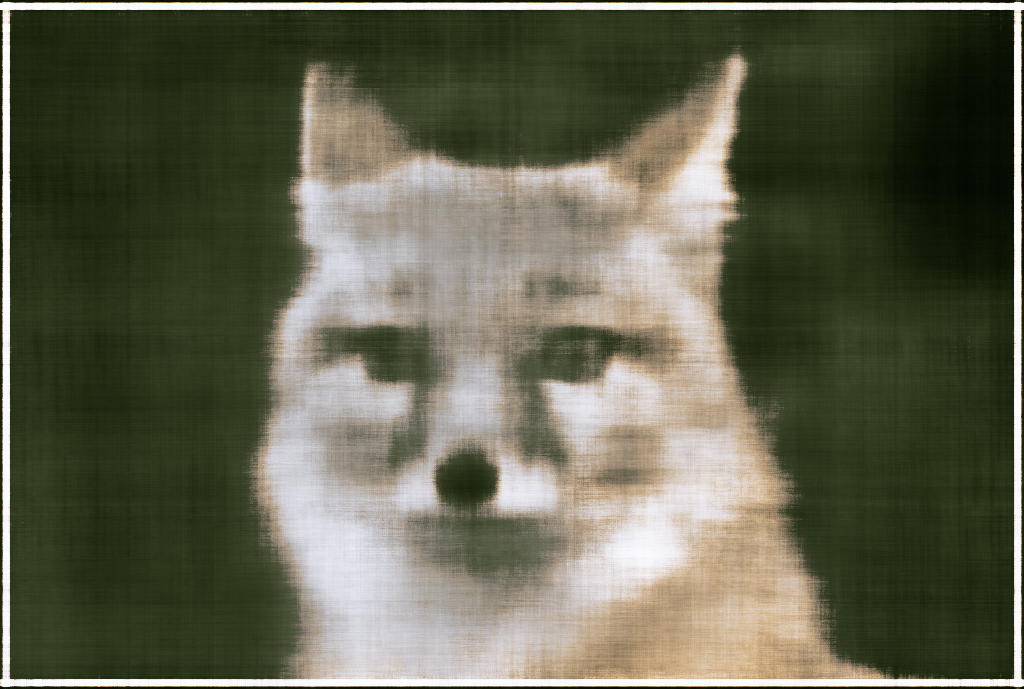
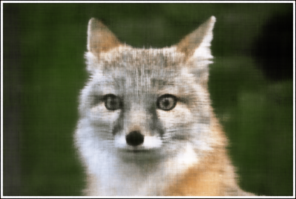
Example: Training progression
Resolution: Pixel Width: 1.024, Pixel Height: 689.
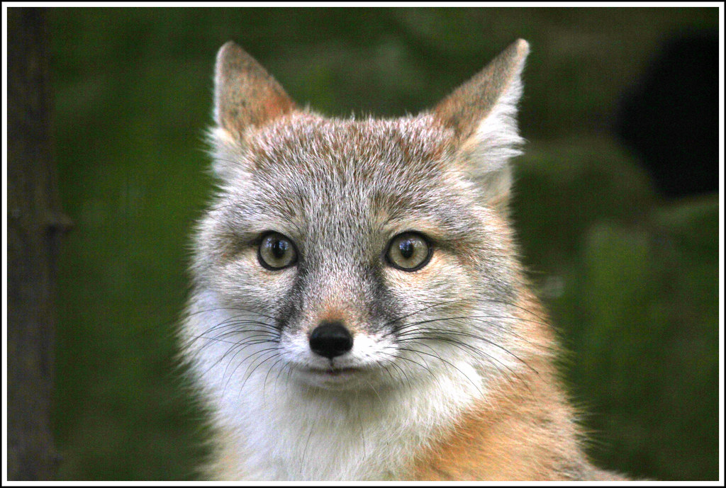
Input image

Step 1
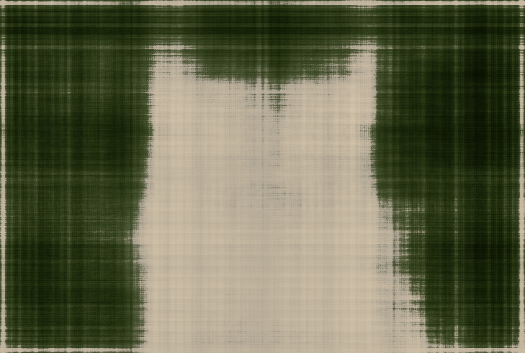
Step 50
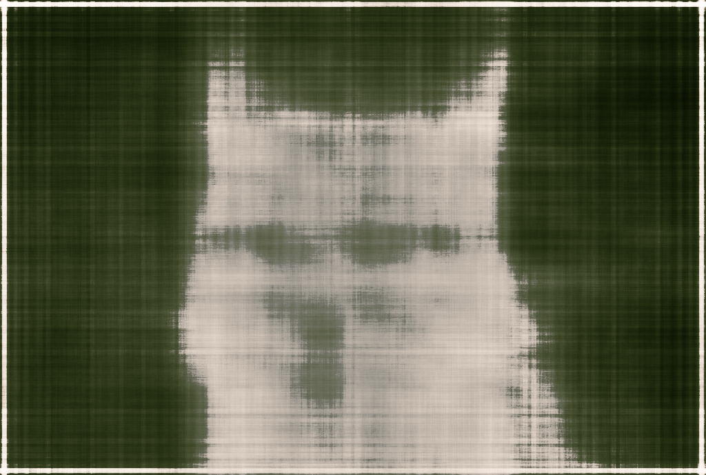
Step 100
Step 200
Step 400
Step 2000
Example: PSNR and MSE curves
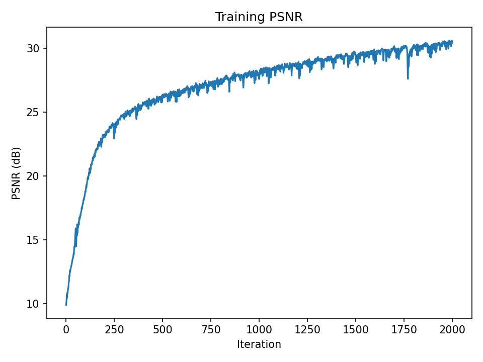
PSNR over iterations
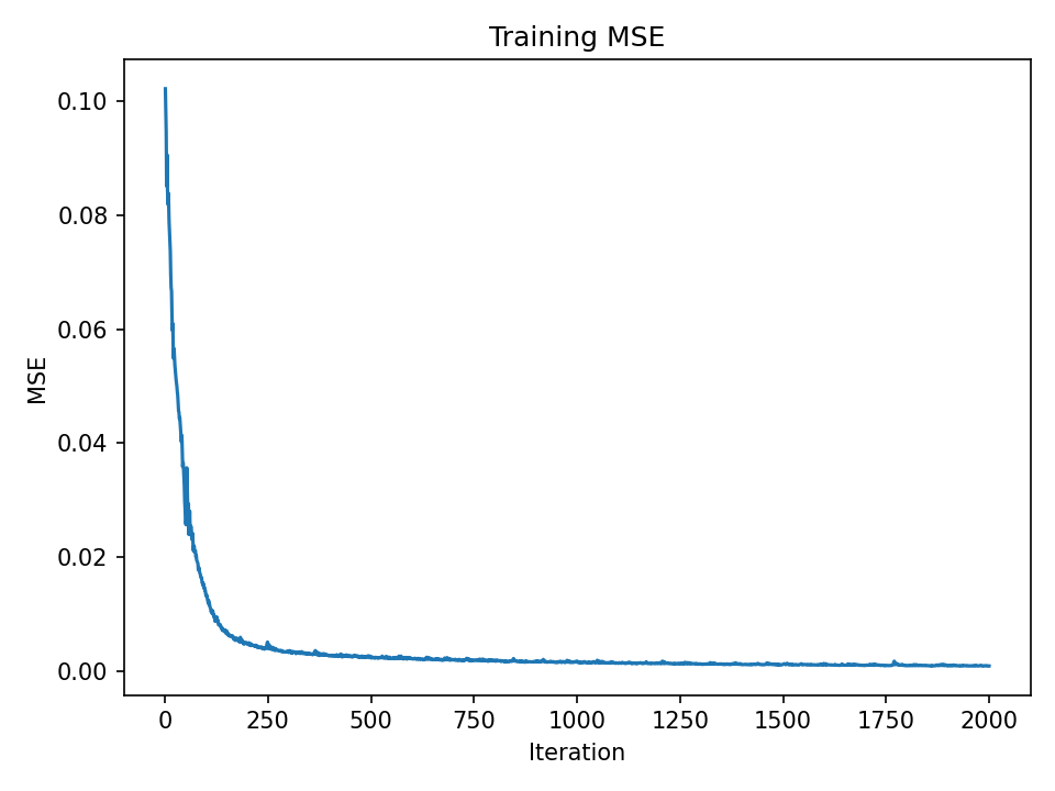
MSE over iterations
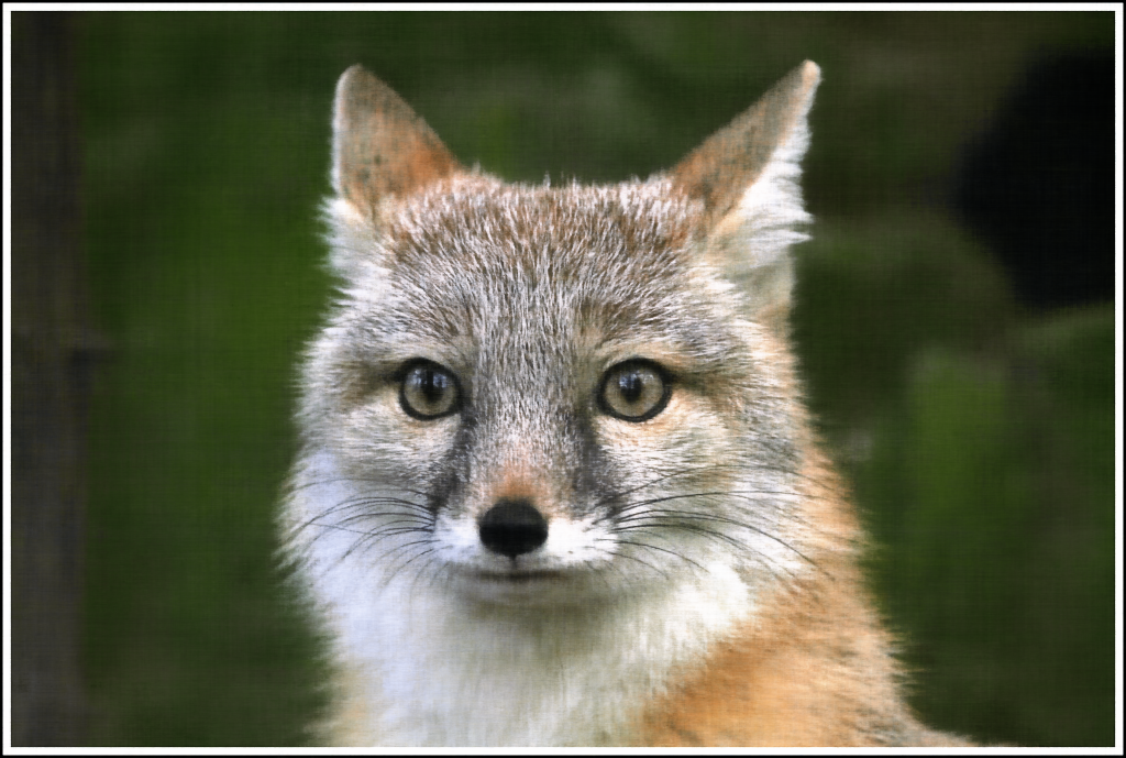
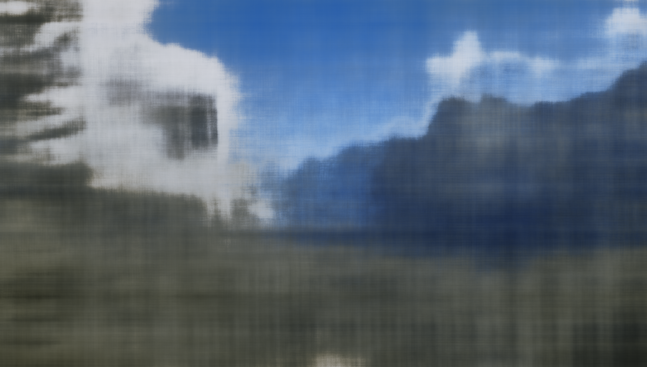
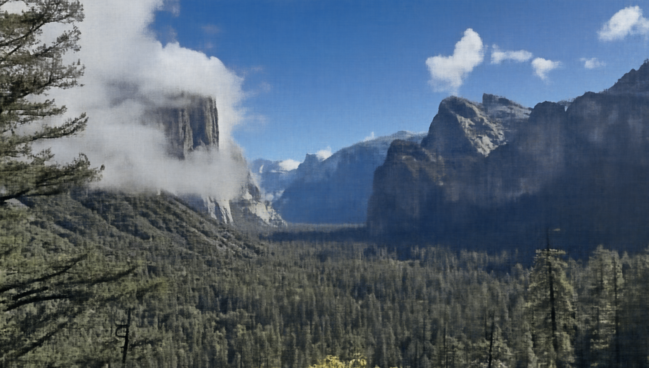
Yosemite: Training progression
Resolution: Pixel Width: 2.075, Pixel Height: 1.177.

Input image

Step 1
Step 200
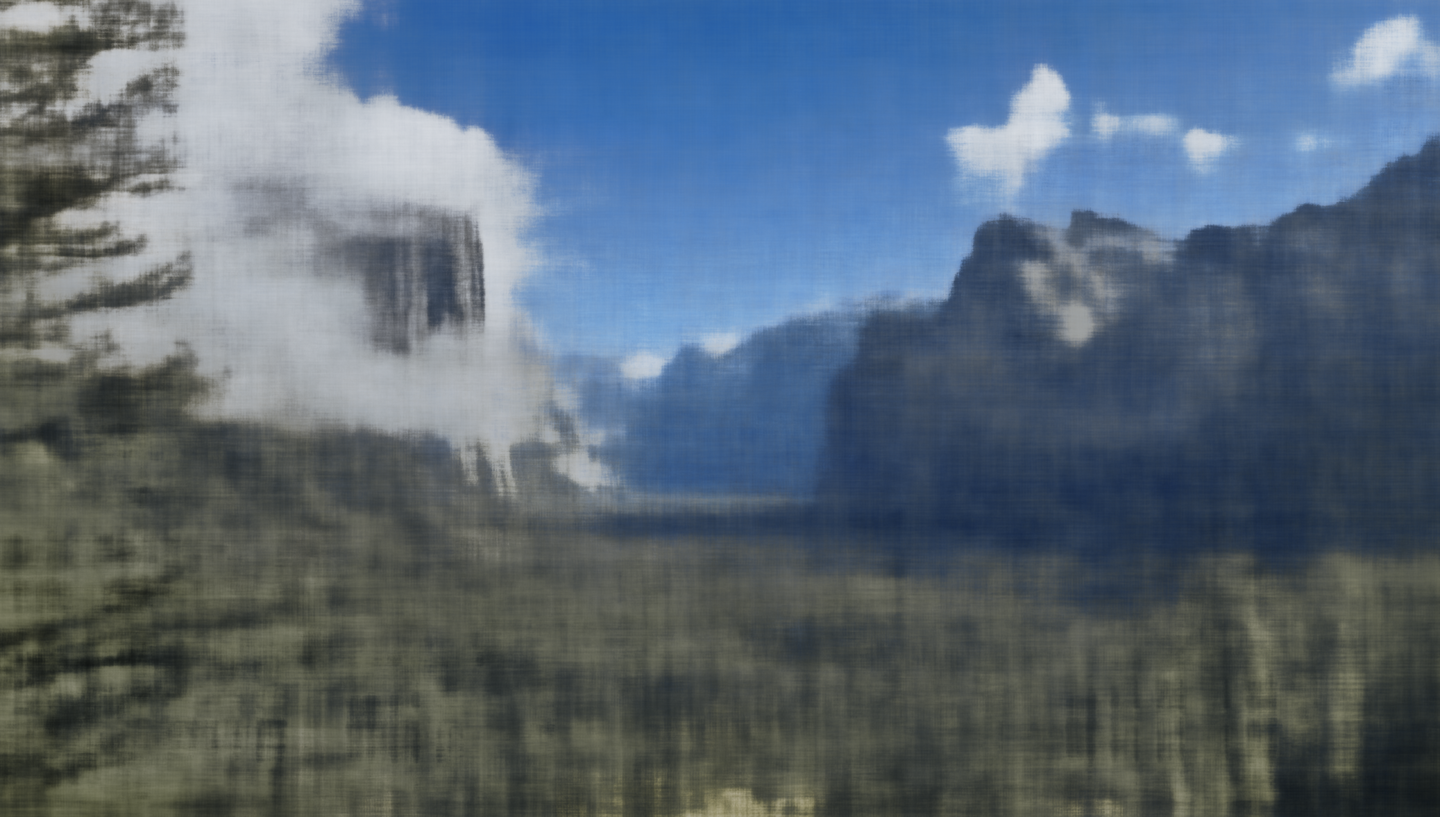
Step 400
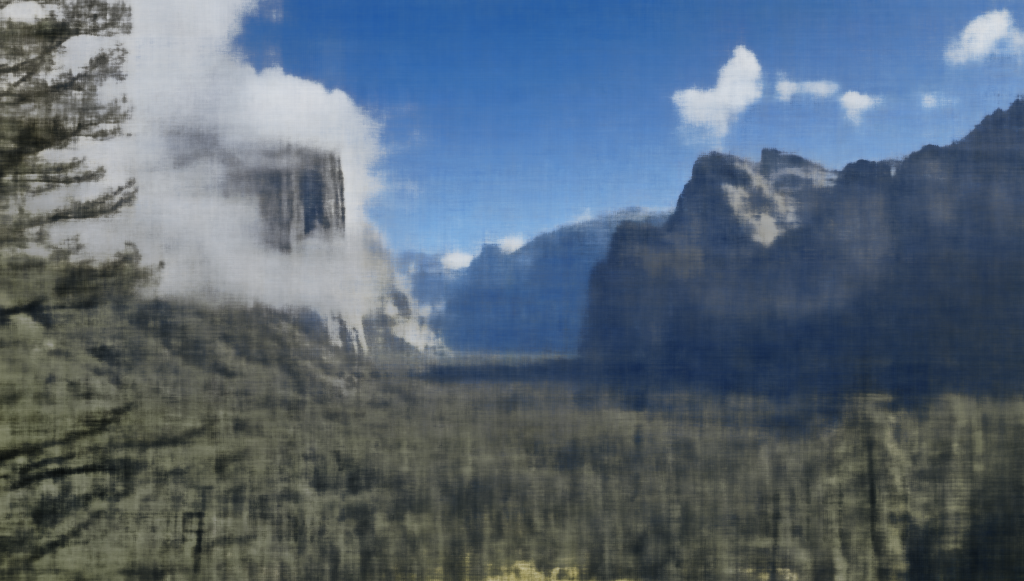
Step 600
Step 1400

Step 7000
Yosemite: PSNR and MSE curves
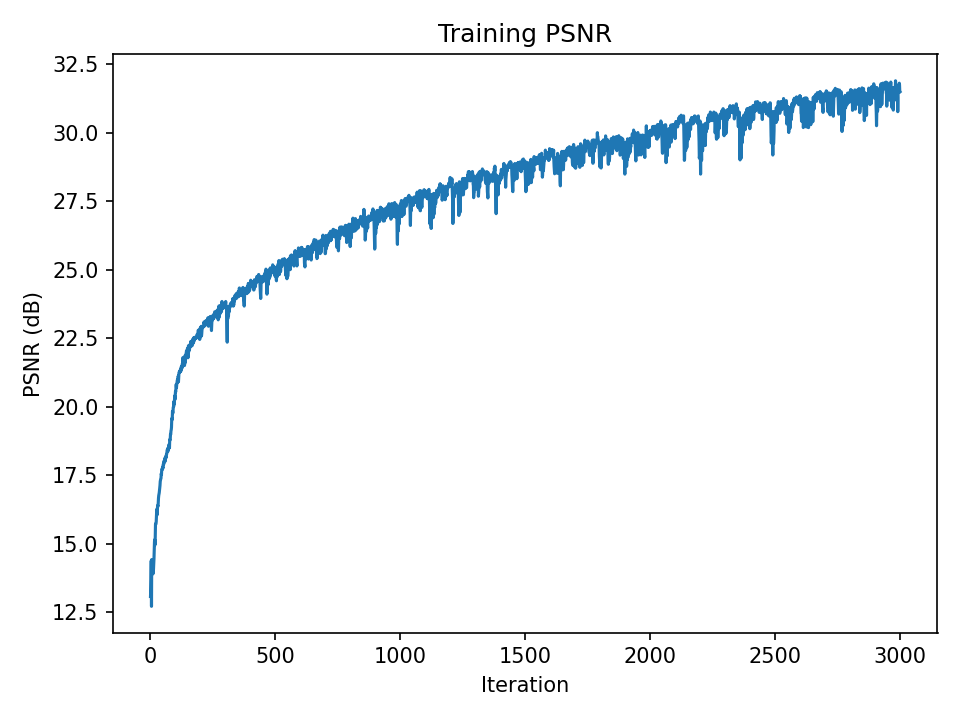
PSNR over iterations
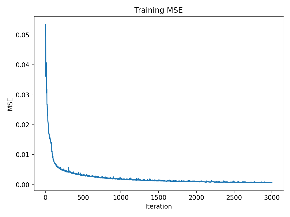
MSE over iterations
Hyperparameter Comparison
- image:
example.jpg - sweep_widths:
32, 64 - sweep_pe_levels:
2, 4
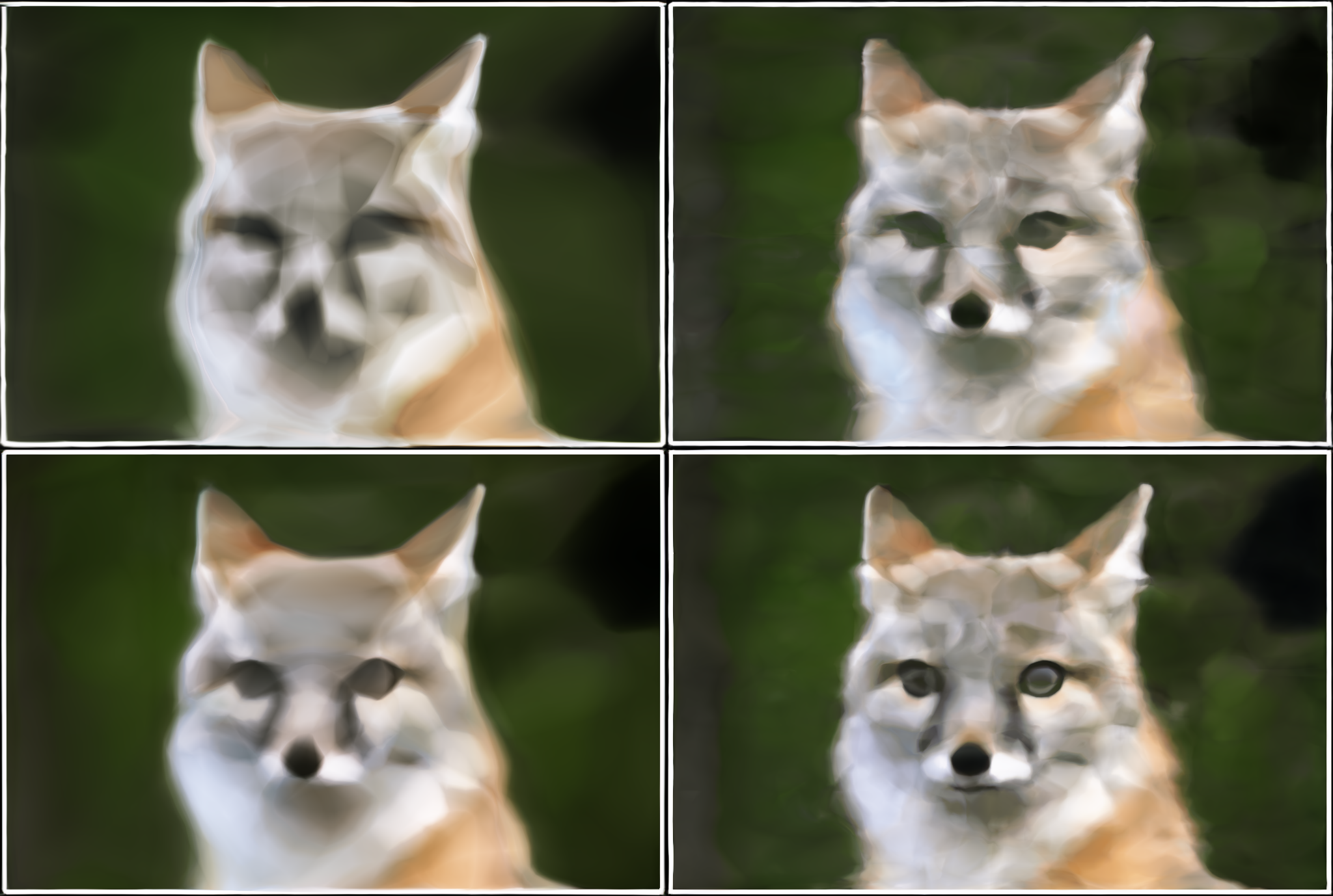
Top-left: w32_L2 • Top-right: w32_L4 • Bottom-left: w64_L2 • Bottom-right: w64_L4
The findings indicate that the network width W and the positional encoding frequency L are both significant. Reconstructions that are excessively smooth or blurry result from the model's lack of frequency coverage and capacity when either is too small. Increasing W gives the network more parameters, increasing capacity and overall image fidelity, and increasing L enables the network to represent higher-frequency detail (less blur).
Part 2: Fit a Neural Radiance Field from Multi-view Images
Part 2.1: Create Rays from Cameras
Implemented the full camera/ray geometry pipeline and data loading used throughout NeRF:
- Loaded a
.npzdataset vianumpy.load, extractedimages_train,c2ws_train, andfocal, and normalized images to[0,1]float32. - Converted camera-space points to world space using homogeneous coordinates and batched matrix multiply, then divided by w with a small clamp for stability.
- Inverted the pinhole model with
K^{-1}[u,v,1]^T(depth scale s applied afterward), precomputingK^{-1}and building homogeneous[u,v,1]per pixel. - Ray origin is the camera center (
c2w[:3,3]). Pixels are mapped to world-space points at unit depth, thenray_d = normalize(x_w − ray_o), with everything fully batched.
Part 2.2: Sampling
Sampled both rays and 3D points along each ray:
- An infinite generator returns batches of
(ray_o, ray_d, pixel_color). Randomly sampled image indices and pixel coordinates, gathered RGB targets, selected per-pixelKandc2w, and called pixel→ray to get batched origins and directions. - Used stratified sampling between
[near, far]withnum_samplesbins. With perturbation, added uniform noise within each interval and returned the 3D points, unit directions, andstep_size = (far − near)/num_samples.
Part 2.3: Putting the Dataloading All Together
The combined pipeline produces per-batch ray origins/directions and colors, and I added a small visualization script (Viser) to render cameras, rays, and sampled 3D points for sanity checks.
Lego dataset: sampled camera rays
Lego dataset: points sampled along rays
Part 2.4: Neural Radiance Field
Implemented a NeRF-style MLP conditioned on positional encodings of 3D points and view directions:
- Used sin/cos bands with frequencies
2^k π, concatenated with the input. Separate levels for positions and directions. - A stack of fully-connected layers (configurable depth/width) with a skip connection that concatenates the encoded position mid‑network.
- Mapped hidden features to
σviasoftplus(with positive bias) for stable, non‑negative densities. - Produced a feature, concatenated encoded view direction, and output RGB with
sigmoidto constrain[0,1].
NeRF Model Architecture
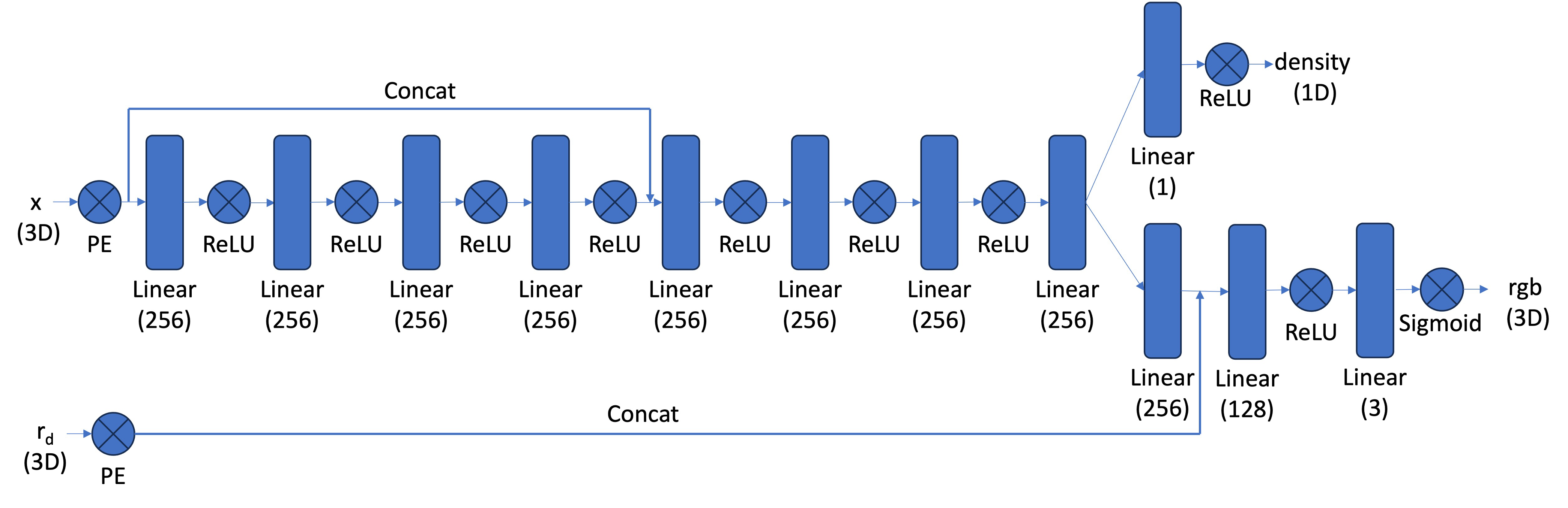
Coarse-to-fine MLP with positional encodings, density head (ReLU) and color head (Sigmoid) conditioned on view direction.
For Part 2 I kept the architecture essentially the same as the reference NeRF: a stacked MLP with a skip connection, separate density and color heads, and positional encodings for both 3D coordinates and view directions. My changes focused on hyperparameters only (e.g., network width, coordinate positional-encoding levels L, and view-direction encoding levels Ldir).
Part 2.5: Volume Rendering
Implemented the discrete volumetric rendering equations in PyTorch for color, depth, and opacity:
- Given per-sample densities σi and colors ci with uniform Δ, computed αi = 1 − exp(−σi Δ) and transmittance Ti = exp(−∑j<i σj Δ). The weights are wi = Ti αi and the rendered color is ∑ wi ci.
- Reused the same weights to compute accumulated opacity acc = ∑ wi and expected depth ∑ wi ti / max(acc, ε).
- Used exclusive cumulative sums for Ti, included shape checks, and ensured full differentiability.
Hyperparameters (Lego NeRF)
| Parameter | Value |
|---|---|
| steps | 10000 |
| width | 256 |
| depth | 8 |
| skip_layer | 4 |
| posenc_L | 10 |
| direnc_L | 4 |
| lr | 0.0005 |
| batch_rays | 4096 |
| num_samples | 64 |
| near | 2.0 |
| far | 6.0 |
Using the standard NeRF model size for Lego (width 256, positional-encoding L=10); other settings as listed.
Actual Lego training ran for 10,000 steps.
Lego: Training progression
Step 1
Step 200
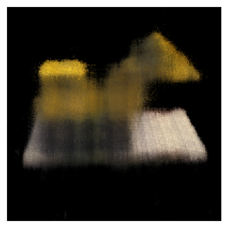
Step 400
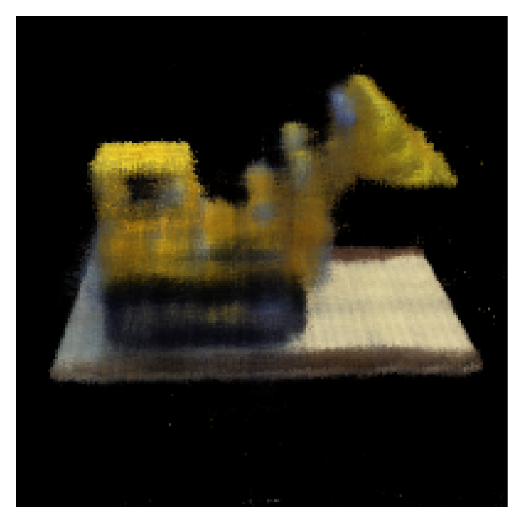
Step 1400
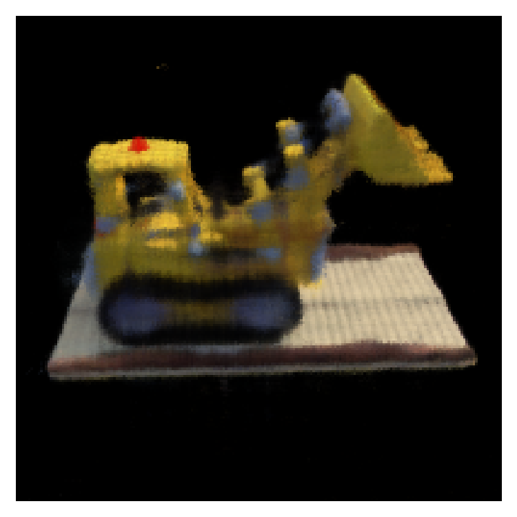
Step 4000
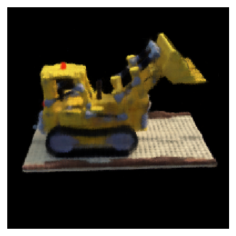
Step 10000
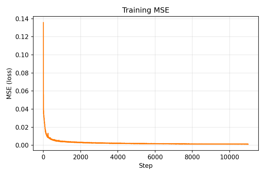
Lego: PSNR and MSE curves
PSNR over iterations
MSE over iterations
Lego: Spherical rendering (10,000 iterations)
Rendered with provided test camera extrinsics after 10,000 iterations.
Part 2.6: Training with your own data
Training ties all components together: per‑step I sample rays and 3D points, run the NeRF, volume‑render, compute MSE against ground‑truth pixels, and optimize with Adam. I log PSNR (−10 log10(MSE)), periodically render full images (with optional depth/opacity), and save checkpoints.
I trained a NeRF on my Part 0 dataset, rendered a circling camera GIF, and tracked loss with intermediate renders.
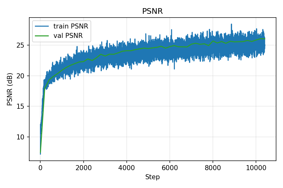
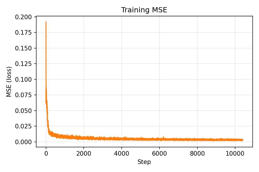
During training, the training MSE continued to decrease while the validation error largely stagnated. This behavior is consistent with the earlier observation that my calibration is not perfectly accurate—validation rays are evaluated under slightly mismatched intrinsics/poses. Even though the validation curves did not keep improving, the rendered reconstructions still looked progressively better to a human observer, suggesting that the model was learning a useful representation of the scene despite these imperfections.
I rescaled images to a width of 800 px and scaled the camera intrinsics accordingly. I chose a higher resolution because my calibration was not perfect: in Viser, back‑projected rays from the camera origin did not intersect exactly at the ArUco tag borders (as they would with ideal intrinsics/poses). My hypothesis was that a higher resolution would reduce pixel‑level quantization error and provide more samples per object area, helping NeRF tolerate small calibration errors. In practice, training at the higher resolution produced better results, which likely supports this rationale (with the trade‑off of increased compute).
Hyperparameters (Own dataset training)
| Parameter | Value |
|---|---|
| steps | 30000 |
| near | 0.2 |
| far | 0.6 |
| batch_rays | 8000 |
| num_samples | 64 |
| width | 512 |
| depth | 8 |
| skip_layer | 4 |
| posenc_L | 12 |
| direnc_L | 4 |
| lr | 6e-4 |
Because I increased the input resolution, rays sampled the scene more densely and the images contained
higher spatial frequencies. To model this additional detail, I raised the positional‑encoding levels
(posenc_L for coordinates and direnc_L for view directions), and increased the network
width to provide more capacity. In short: more pixels → more high‑frequency content → higher PE,
and denser 3D sampling → a wider MLP to faithfully represent the added detail.
Own dataset: Training progression

Step 1
Step 200
Step 400
Step 1400
Step 4000

Step 10000
Own dataset: PSNR and MSE curves
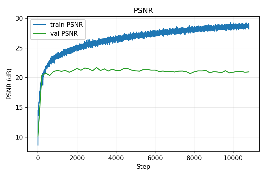
PSNR over iterations (train/val)
MSE over iterations (train/val)
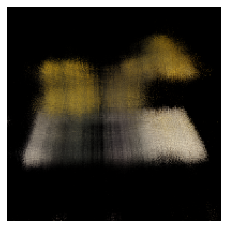
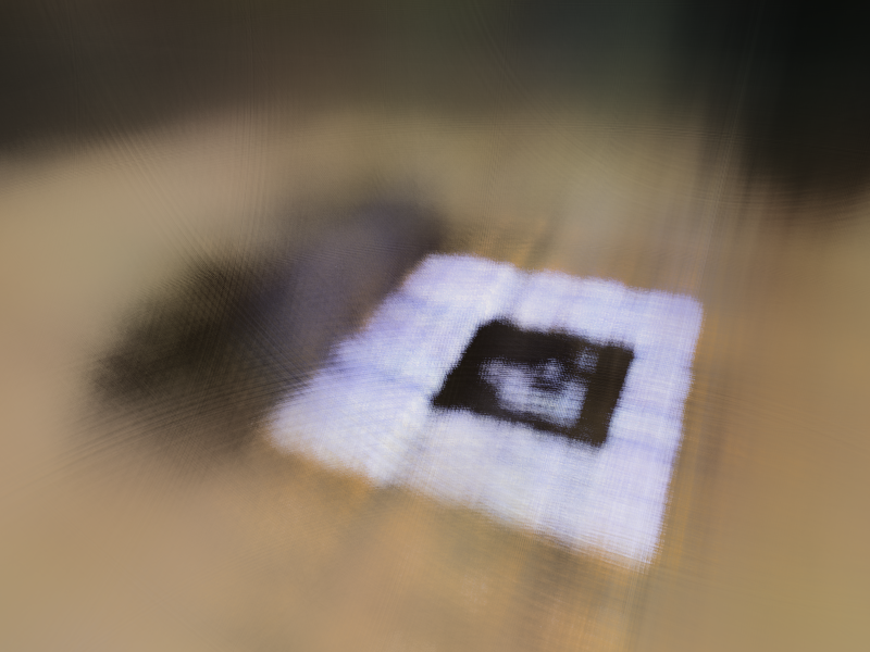
Own dataset: Shoe novel views
Shoe reconstruction, 24-frame spin.
Bells & Whistles
Depth Map Rendering with Accumulated Opacity Threshold
Along each camera ray, NeRF samples points with predicted densities σ (and colors). Volumetric rendering assigns each sample an opacity αi = 1 − exp(−σi Δi) over interval Δi and a transmittance Ti = exp(−∑j<i σj Δj). The per‑sample weight is wi = Ti · αi. The depth map is the ray‑wise expectation of distance: Depth = ∑ wi · ti (optionally normalized for display).
The accumulated opacity (confidence) that a ray intersects a surface is
acc = ∑ wi, with values near 0 indicating empty space and near 1 indicating an
opaque hit. A threshold acc_thresh masks rays with insufficient confidence
(acc < acc_thresh) and normalizes depths over the remaining pixels, suppressing floaters and
background leakage in low‑confidence regions.
I tuned acc_thresh empirically. Lower values kept semi‑transparent floaters, while higher values
started knocking out thin structures. Settling around acc_thresh ≈ 0.3 consistently produced cleaner,
more stable depth maps for my scenes.
Lego: Depth Map Comparison
Without acc_thresh (noisy, shows floaters and artifacts)
With acc_thresh = 0.3 (clean, artifacts removed)
Learnings
- Dataset creation was the hardest part. Reliable intrinsics/poses and disciplined capture matter more than small model tweaks.
- Lego trained easily; my own data was more challenging. High‑quality results required precise calibration and consistent capture geometry.
- Surprisingly, skipping undistortion improved my results—likely because the iPhone lens has minimal distortion and/or applies in‑camera correction.