Project 5 – Diffusion Models (Part A)
CS180/280A: Intro to Computer Vision and Computational Photography
Setup & Playing with DeepFloyd IF
Diffusion models generate images by iteratively denoising noise; in Part A, results come from the pretrained DeepFloyd IF text‑to‑image model (Stage I + Stage II). Access was configured on Hugging Face and prompt embeddings were generated on the course clusters. A fixed random seed (1234) is used throughout Part A for reproducibility.
For text‑to‑image sampling, I compared the default num_inference_steps=20 against a longer run with
num_inference_steps=50 (see the 50‑step results below).
The 50‑step outputs look noticeably more realistic and coherent, with finer‑grained texture and fewer artifacts.
This makes sense because more inference steps means more iterative denoising/refinement updates, so the model has more chances
to add detail and clean up structure.
However, longer runs are slower and cost more compute. For simplicity and faster iteration (especially under limited compute), I used 20 steps for the remaining parts of the assignment.
Qualitatively, the samples also depend on the prompt: short, precise prompts describing well‑known concepts tend to work best and produce very faithful images. In contrast, longer and more specific prompts often performed worse here, likely because those detailed combinations are less consistently represented in the training distribution.
Below are example prompts and their Stage II upsampled samples.
- Created a Hugging Face account, accepted the
DeepFloyd/IF-I-XL-v1.0license, and logged in via access token. - Generated custom text prompt embeddings on the course clusters and saved them as a
.pthfile for Colab.
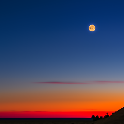
photo of the moon.
a rocket ship.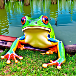
big frog near a lake.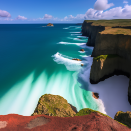
a rocky coastline.Same prompts with 50 inference steps
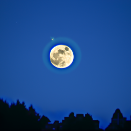
photo of the moon.
a rocket ship.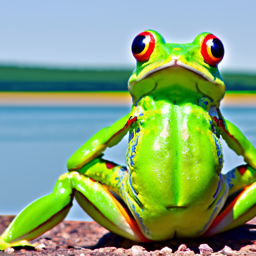
big frog near a lake.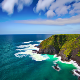
a rocky coastline.Forward Process: Noising the Campanile
The forward diffusion process was implemented:
\(x_t = \sqrt{\bar\alpha_t}\,x_0 + \sqrt{1-\bar\alpha_t}\,\epsilon\),
where \(\bar\alpha_t\) is given by the DeepFloyd schedule and \(\epsilon \sim \mathcal{N}(0,I)\).
Using the provided alphas_cumprod, increasing t produces progressively noisier versions of the Campanile.


Classical Gaussian Denoising
Before using diffusion models, the forward‑noised Campanile images were denoised with Gaussian blur
(via torchvision.transforms.functional.gaussian_blur). Kernel size and \(\sigma\) were tuned for each noise level,
but even the best results blur out fine details and cannot fully remove structured noise.
At higher timesteps the noise dominates and overlaps with true image edges, so a low‑pass filter cannot separate “noise” from “signal”: increasing \(\sigma\) suppresses noise but also wipes out high‑frequency detail, producing blurry and distorted results.
Highlighted below are the settings that looked best: \(\sigma=1.0\) for \(t=250\), \(\sigma=2.0\) for \(t=500\), and \(\sigma=2.0\) for \(t=750\).
t = 250


t = 500


t = 750


One‑Step Denoising with DeepFloyd
The pretrained Stage I UNet (stage_1.unet) is used (conditioned on the text embedding for
“a high quality photo”) to predict noise in a single step, then \(x_0\) is computed from \(x_t\) and \(\epsilon_\theta(x_t, t)\)
using the closed‑form denoising formula.


Iterative Denoising with Strided Timesteps
A strided schedule from \(t=990\) down to \(0\) (stride 30) is used, together with an iterative_denoise
loop that repeatedly predicts the clean image, interpolates between signal and noise, and adds the model’s learned variance.
Compared to one‑step denoising or Gaussian blur, the iterative sampler produces much cleaner reconstructions.
Given a current timestep \(t\) and the next (less noisy) timestep \(t'\), the strided DDPM update is:
\[ x_{t'}=\frac{\sqrt{\bar{\alpha}_{t'}}\,\beta_t}{1-\bar{\alpha}_t}\,x_0 \;+\; \frac{\sqrt{\alpha_t}\,(1-\bar{\alpha}_{t'})}{1-\bar{\alpha}_t}\,x_t \;+\; v_\sigma \]


Intermediate steps (iterative denoising)
Snapshots of the reconstruction as the iterative sampler progresses from a noisy start state toward a clean image.


Sampling from Pure Noise
With i_start = 0 and a pure Gaussian noise input, the iterative sampler becomes a text‑to‑image generator.
Below are samples for the prompt “a high quality photo” using the same seed and diffusion schedule.


Classifier‑Free Guidance (CFG)
The sampler is extended to perform Classifier‑Free Guidance by running the UNet twice per step (with conditional and unconditional text embeddings) and combining the noise estimates as \(\epsilon_{\text{CFG}} = \epsilon_{\text{uncond}} + s\cdot(\epsilon_{\text{cond}} - \epsilon_{\text{uncond}})\). A moderate guidance scale dramatically improves adherence to the prompt at the cost of diversity.


Image‑to‑Image Translation (SDEdit)
Using the forward process to add noise and then running iterative CFG‑guided denoising lets the model “edit” an existing image while preserving its coarse structure. Lower noise levels make subtle edits, while higher levels push the image closer to a fresh sample from the text‑conditioned manifold.
Campanile edits with different starting indices


Edits of my own test images
Example 1


Example 2


Editing Hand‑Drawn & Web Images
SDEdit works especially well when starting from non‑photographic inputs (sketches) and web images. The diffusion model hallucinates natural textures while loosely preserving the layout of the input.
Web image example (apple)


Hand‑drawn example 1


Hand‑drawn example 2


Inpainting via Diffusion
For inpainting, denoising is repeated while clamping pixels outside the masked region back to a noisy version of the original image. This follows the RePaint strategy and lets the model “fill in” missing content while keeping the context fixed.
Campanile inpainting – run 1


Campanile inpainting – run 2


Campanile inpainting – run 3


Text‑Conditional Image‑to‑Image Translation
Finally, SDEdit is combined with stronger text prompts to steer the edits: instead of simply projecting back to the “natural image manifold,” the model is guided toward images that both resemble the original and match a new description (e.g., turning a landmark into a “rocket ship” scene).
Example 1 – “big frog near a lake” → Campanile


Example 2 – “a rocket ship” → Bryce Canyon


Example 3 – “big frog near a lake” → Car


Example 4 – “photo of the moon” → Taipei skyline


Example 5 – “a rocket ship” → Campanile


Visual Anagrams
To create visual anagrams, an image is jointly denoised upright and rotated by 180°, using two different prompts and averaging the noise estimates (flipping back the rotated one). The resulting image looks like one concept upright and another when flipped upside‑down.
Concretely, at each step \(t\) two CFG noise estimates are computed and averaged:
\[ \epsilon_1=\text{CFG}(\text{UNet}(x_t,t,p_1)),\quad \epsilon_2=\text{flip}(\text{CFG}(\text{UNet}(\text{flip}(x_t),t,p_2))),\quad \epsilon=\frac{\epsilon_1+\epsilon_2}{2}. \]
Example 1 – ‘an oil painting of an old man’ / ‘an oil painting of people around a campfire’


Example 2 – ‘a painting of a deer’ / ‘a painting of houseplants’


Example 3 – ‘a painting of a fox’ / ‘a painting of a fruit bowl’


Hybrid Images with Factorized Diffusion
Inspired by classical hybrid images, a composite noise estimate is formed by taking low frequencies from one prompt’s noise and high frequencies from another (using Gaussian blur and subtraction). Running the diffusion sampler with this hybrid noise produces images that read as one concept from afar and another up close.
In the examples below, the left prompt supplies the high‑frequency content, and the right prompt supplies the low‑frequency content.
Hybrid Example 1 – High‑freq (left): ‘a lithograph of a skull’ / Low‑freq (right): ‘a lithograph of waterfalls’


Hybrid Example 2 – High‑freq (left): ‘an oil painting of a snowy forest at night’ / Low‑freq (right): ‘a painting of a teddy bear’


Hybrid Example 3 – High‑freq (left): ‘big frog near a lake’ / Low‑freq (right): ‘a surfer surfing a wave’


Extra Visual Anagrams & Custom Logo
For additional visual anagrams, other transformations beyond simple flips are used, such as 90° rotations and intensity inversion, and text‑conditional edits are applied to create a course‑style logo.
Rotation-based visual anagrams
Example 1 – ‘a watercolor painting of a village in the mountains’ / ‘a watercolor painting of a ship at sea’


Example 2 – ‘a painting of a rabbit’ / ‘a painting of a duck’


Intensity-based visual anagrams
Example 1 – ‘a painting of a rabbit’ / ‘a painting of a duck’


Example 2 – ‘a pencil sketch of a cat’ / ‘a pencil sketch of a bicycle’


Logo: text‑conditional image‑to‑image iterations
Prompt: “a simple vector logo of a pixelated eye for UC Berkeley CS 280A”.
Final logo pick
This final logo was chosen because it clearly features an “eye” in the center (the best camera ever) and a pixelation motif, tying directly to computer vision and image representation in this course.
Flow Matching from Scratch!
Part B trains UNet‑based denoisers and flow‑matching models on MNIST, progressing from a single‑step denoiser to time‑ and class‑conditioned iterative generators.
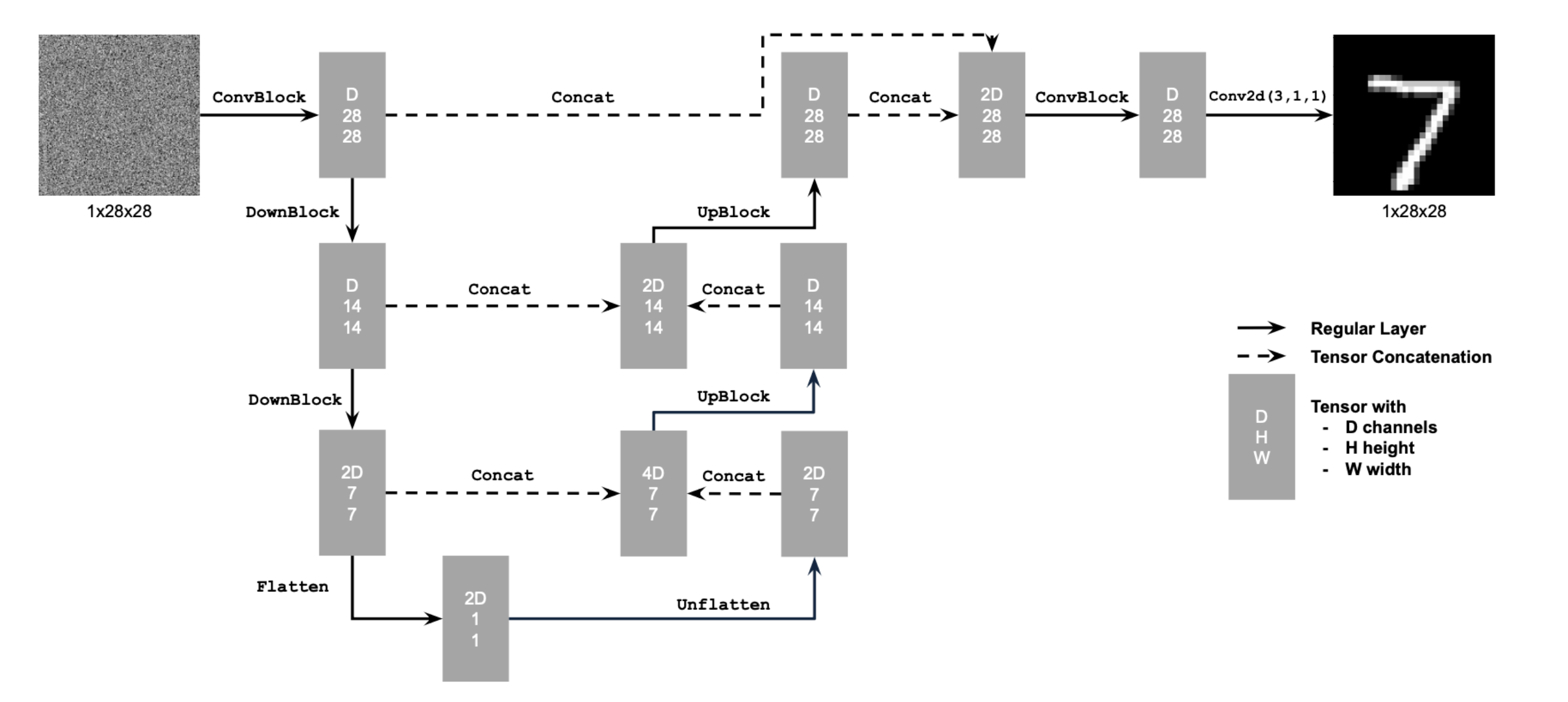
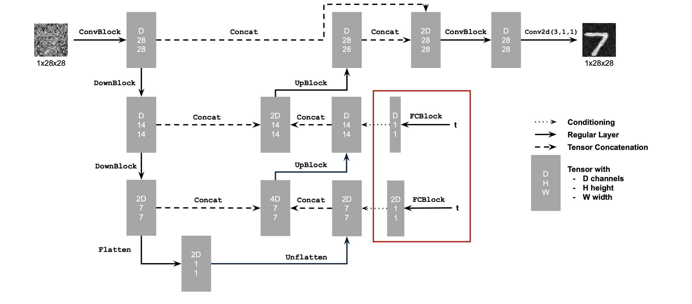
UNet architecture (single‑step denoiser)
The one‑step denoiser uses a standard UNet with downsampling/upsampling blocks and skip connections.
Using the UNet to train a denoiser
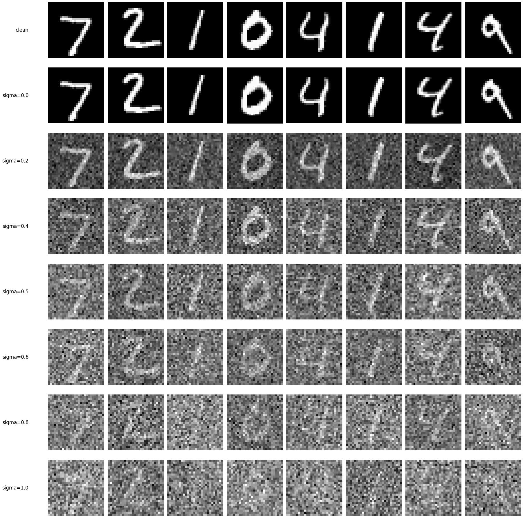
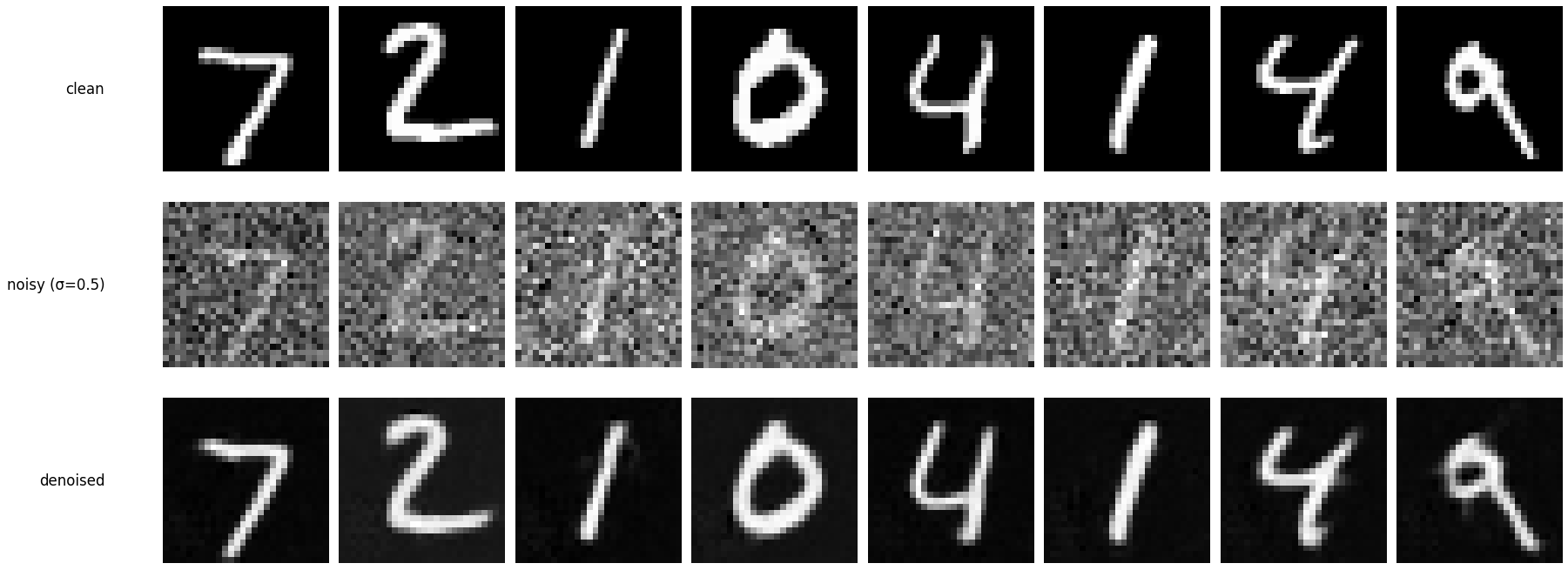
The effect of varying noise level \(\sigma\) on MNIST digits is visualized by directly applying Gaussian noise to clean images.
\[ \mathcal{L}=\mathbb{E}_{z,x}\left[\left\lVert D_{\theta}(z)-x\right\rVert^2\right] \qquad z = x + \sigma \epsilon,\;\;\epsilon \sim \mathcal{N}(0, I). \]
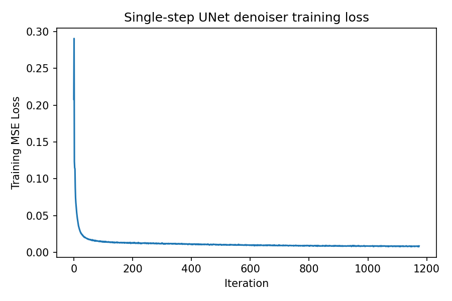
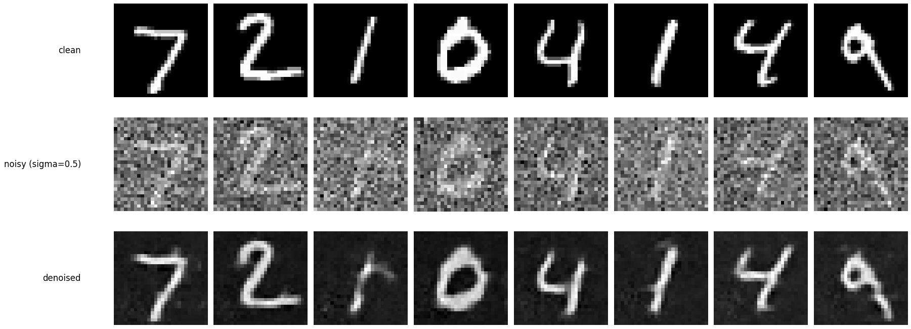
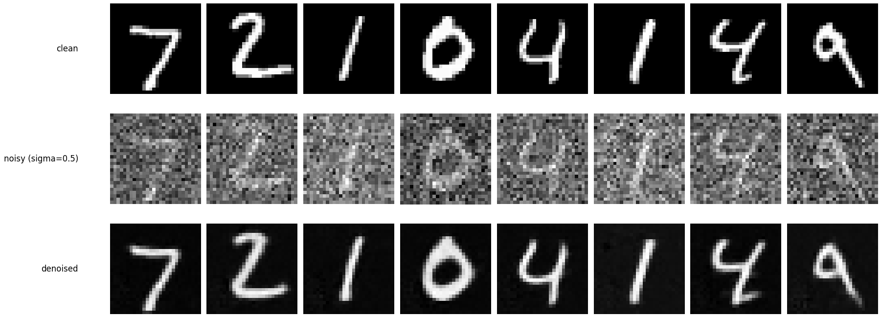
Training a single‑step denoising UNet
The UNet is trained to denoise MNIST digits noised with \(\sigma = 0.5\) using an \(\ell_2\) reconstruction loss.
\[ \mathcal{L}=\mathbb{E}_{z,x}\left[\left\lVert D_{\theta}(z)-x\right\rVert^2\right] \]
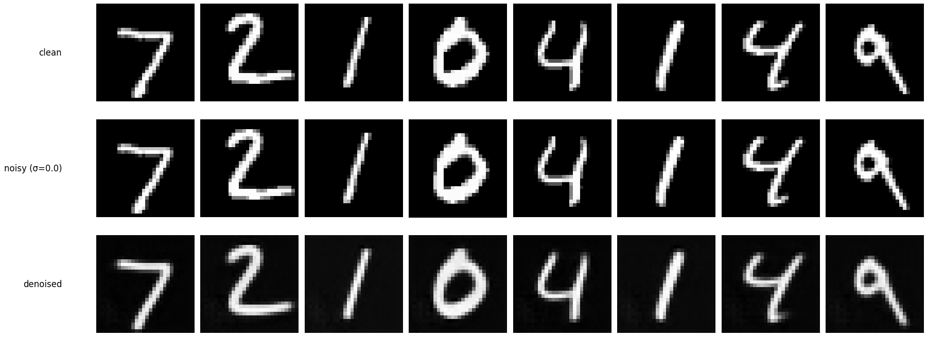
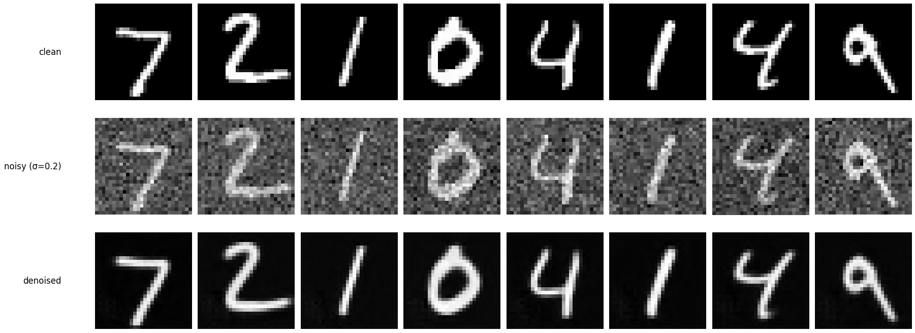
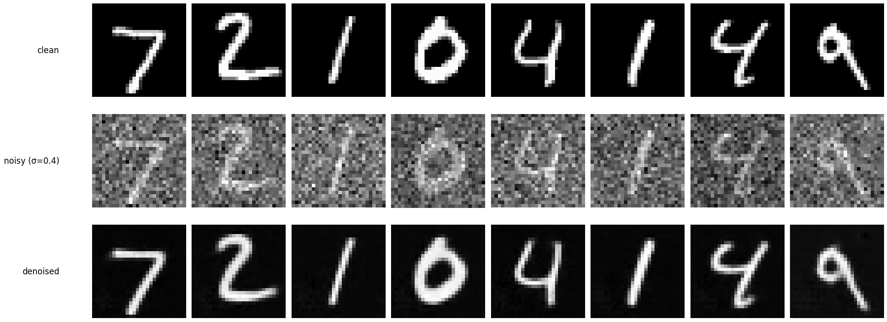
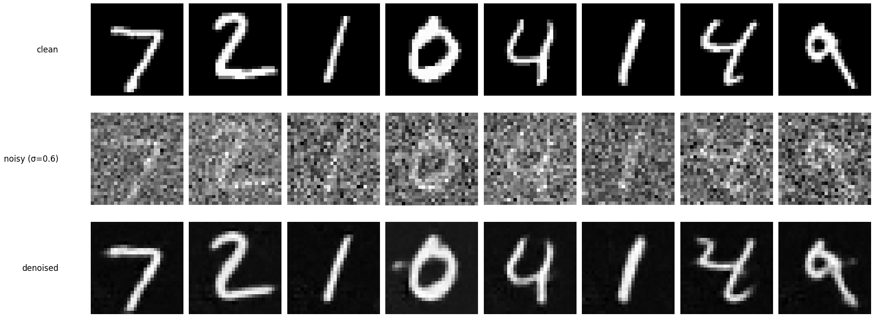
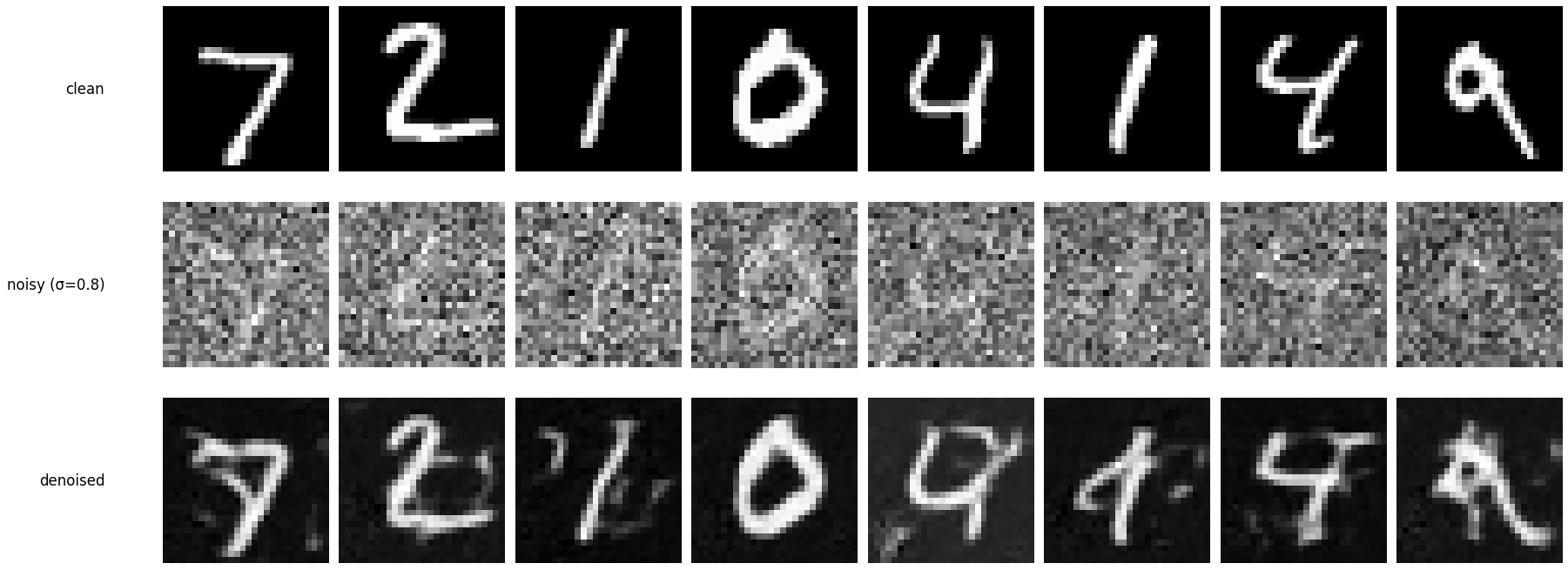
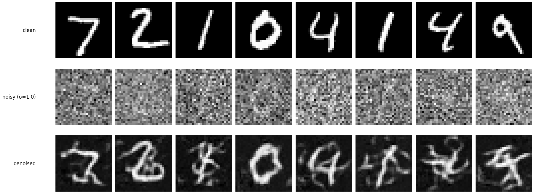
Out‑of‑distribution testing
Holding the same test digits fixed and varying \(\sigma\). The model was trained at \(\sigma=0.5\), so it performs best near that noise level.
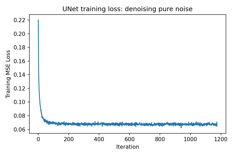
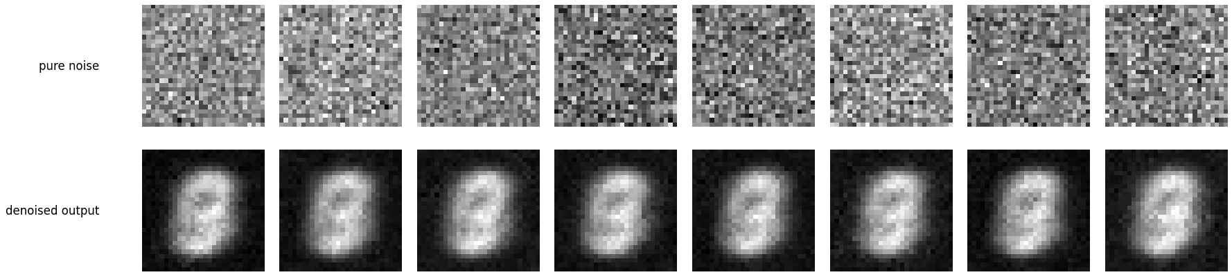
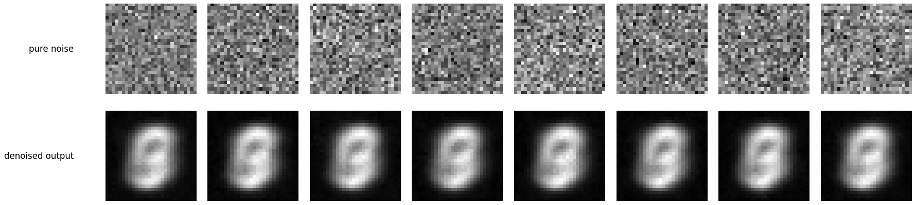
Denoising pure noise
The UNet is retrained to map pure Gaussian noise directly to clean digits. With an MSE loss the model tends to predict “average” digit shapes.
This “average digit” pattern is expected: mapping pure noise to a digit is highly ambiguous (many digits could plausibly fit), and minimizing \(\ell_2\) error encourages the network to output the conditional mean of the training targets. Averaging over multiple digit modes produces a blurry, prototype-like digit rather than a crisp sample from any single class.
Training a flow matching model
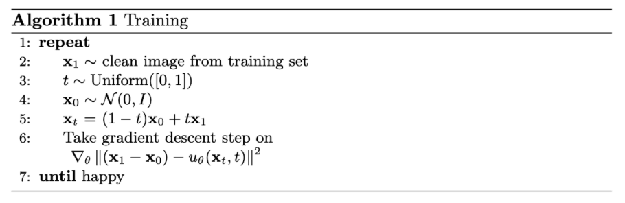
For iterative generation, flow matching is used: interpolate between noise \(x_0\sim\mathcal{N}(0,I)\) and a clean sample \(x_1\), define the flow field, and train a UNet to predict it.
The key difference from the single‑step denoiser is that this model learns a vector field over time. Instead of predicting a clean image directly in one shot, it predicts how to move a sample from the noise distribution toward the data distribution as \(t\) increases.
\[ x_t=(1-t)x_0 + t x_1,\;\; t\in[0,1], \qquad u(x_t,t)=\frac{d}{dt}x_t=x_1-x_0, \] \[ \mathcal{L}=\mathbb{E}_{x_0\sim p_0(x_0),\,x_1\sim p_1(x_1),\,t\sim U[0,1]}\left[\left\lVert (x_1-x_0)-u_\theta(x_t,t)\right\rVert^2\right]. \]
Adding time conditioning to UNet
Scalar time \(t\in[0,1]\) is injected into the UNet via FCBlocks, modulating intermediate feature maps as in the handout.
Intuitively, small \(t\) corresponds to “mostly noise” and large \(t\) corresponds to “mostly data.” Conditioning lets one network share parameters across all timesteps while still behaving differently depending on where along the trajectory the current sample lies.
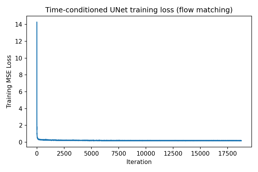
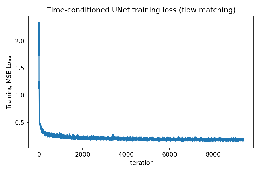
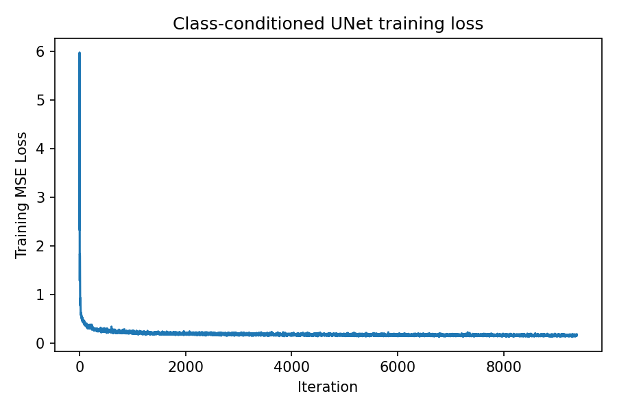
Time‑conditioned UNet training
Training samples \(x_1\), \(t\sim U[0,1]\), and \(x_0\sim \mathcal{N}(0,I)\), constructs \(x_t=(1-t)x_0+tx_1\), and trains \(u_\theta(x_t,t)\) to match \(x_1-x_0\).
Because \(t\) is resampled every iteration, the model sees a continuum of interpolation levels during training. This encourages a smooth flow field and improves stability compared to training on a small fixed set of noise levels.
The loss curve below should decrease as the model learns to predict the correct direction of motion (from noise toward digits). Minor oscillations are expected due to different \(t\) values and batch content.
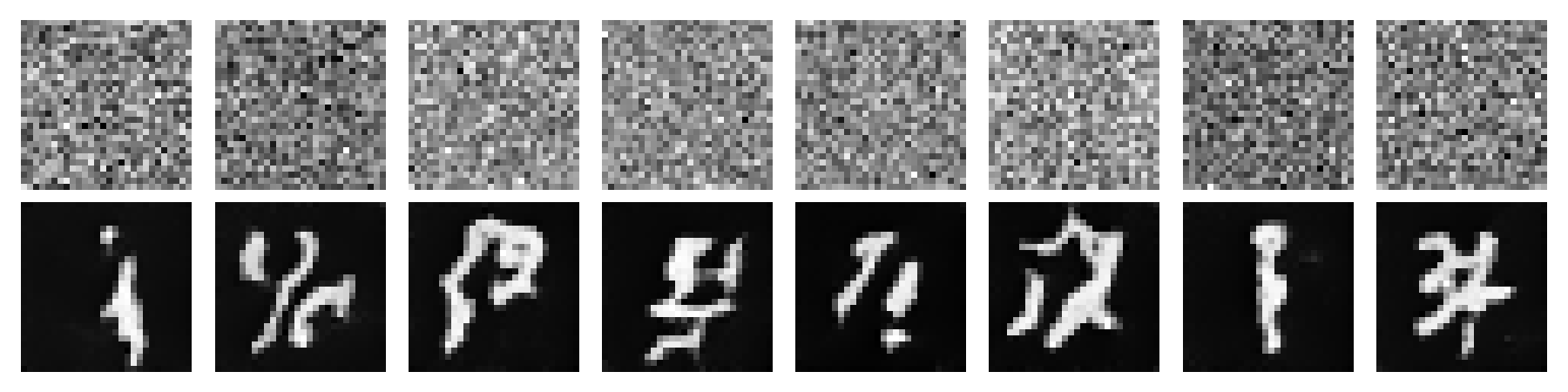
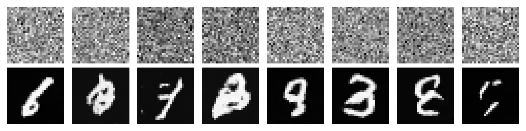
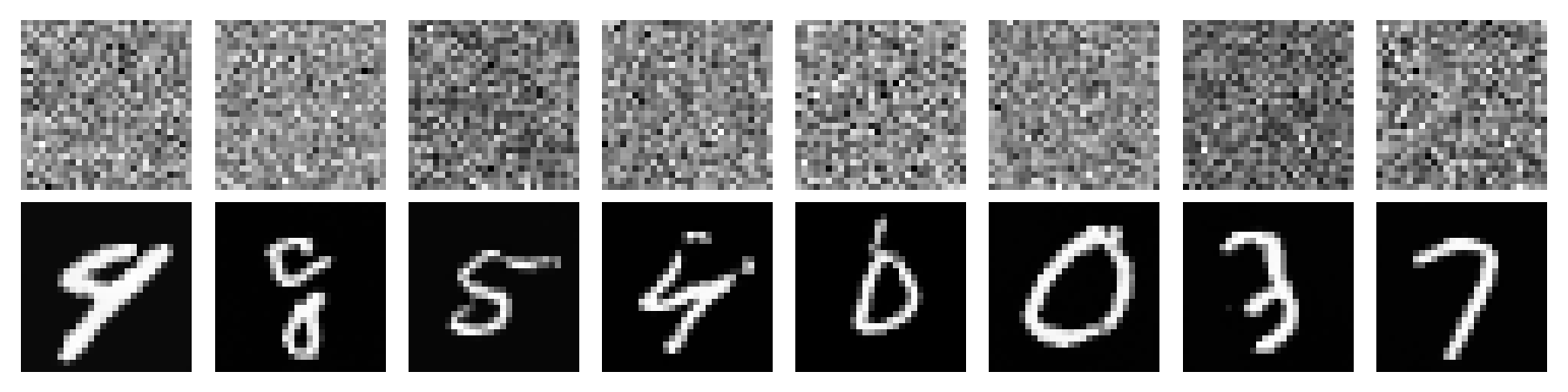
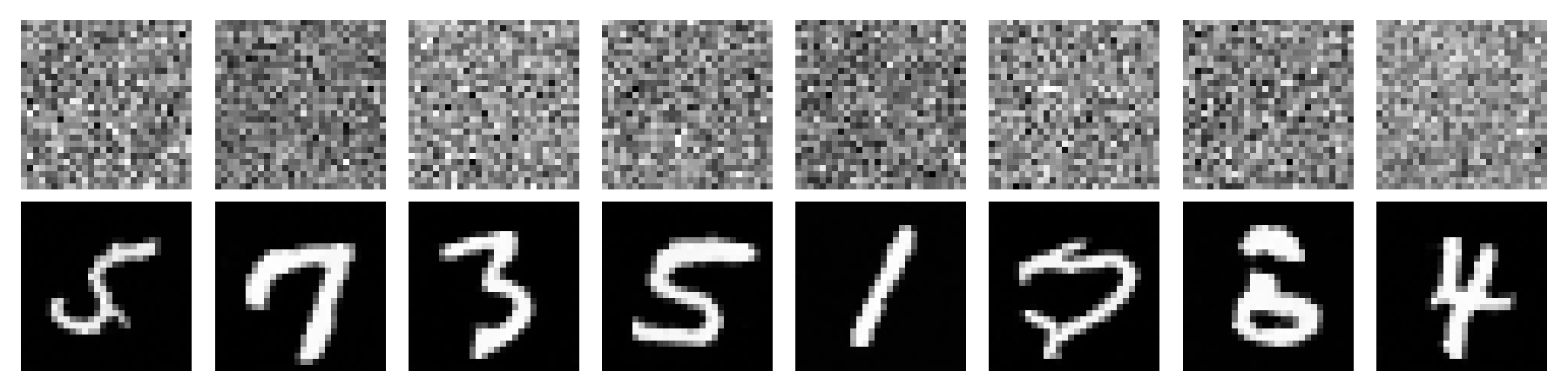
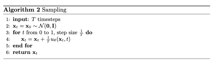
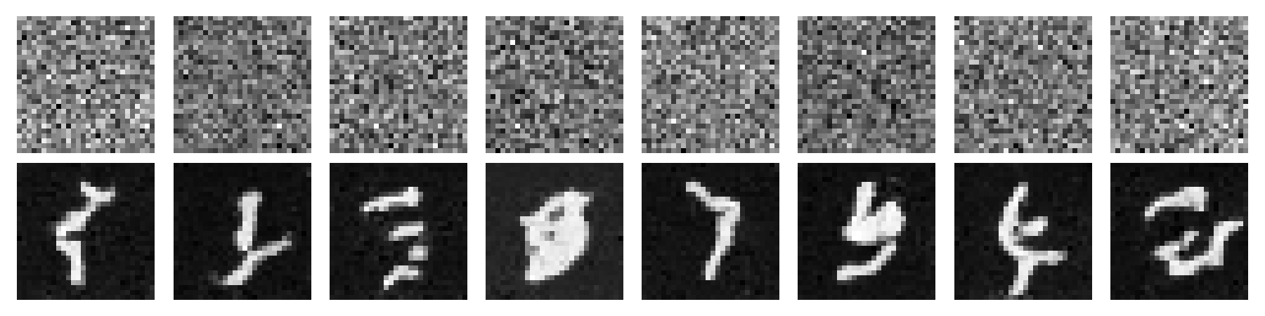
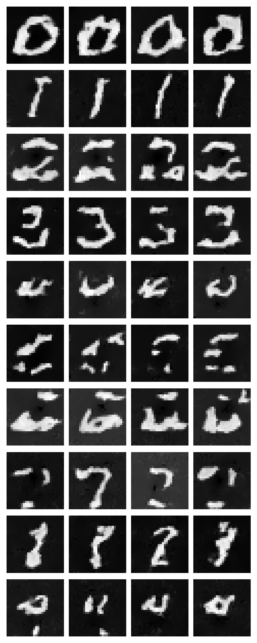
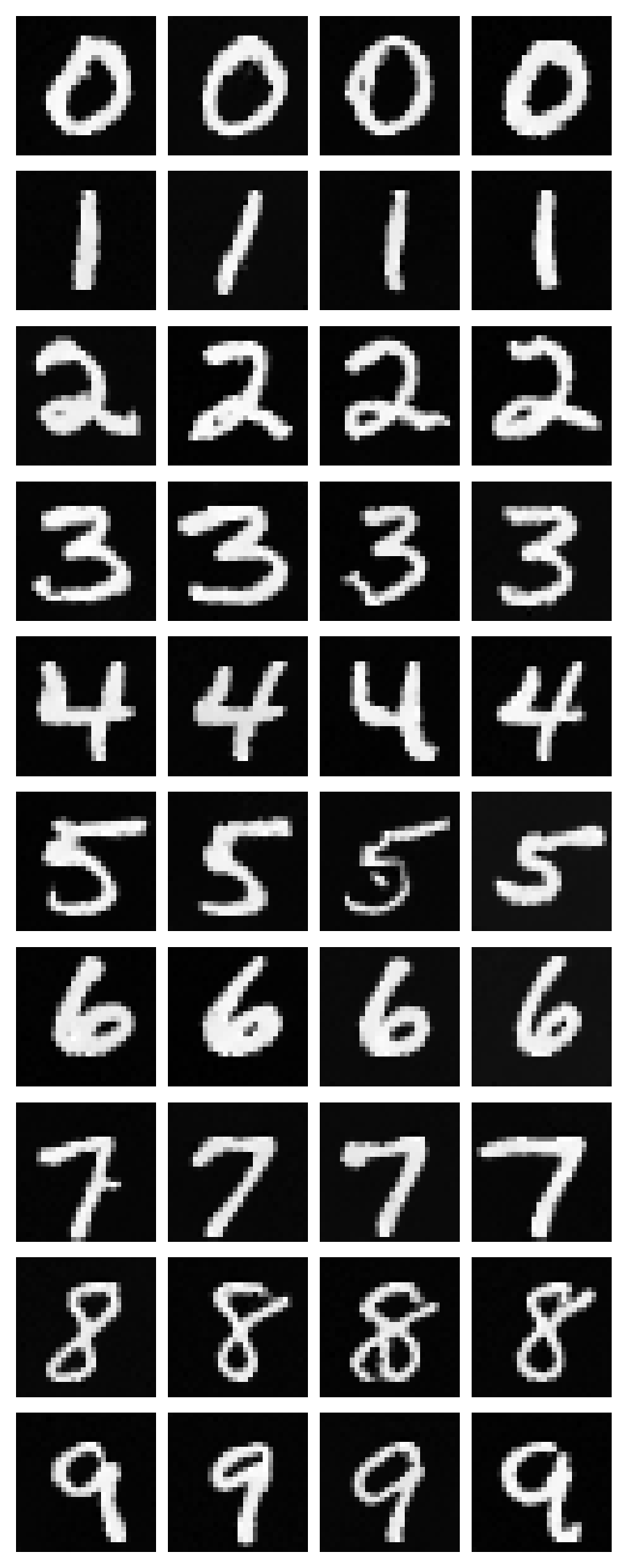
Sampling from time‑conditioned UNet
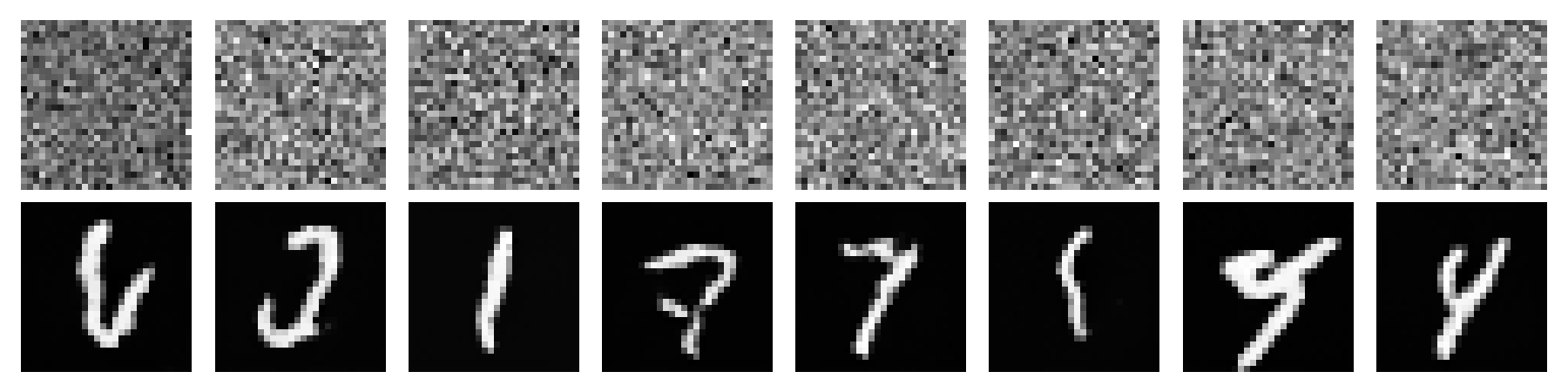
Each image below is a grid of multiple samples (top row: initial noise; bottom row: final generated digits).
Sampling integrates the learned flow from \(t=0\) to \(t=1\) using \(T\) discrete steps (Euler). Early in training (Epoch 1) samples tend to be faint or malformed; by later epochs, digits become higher contrast with clearer strokes.
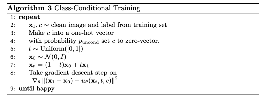
Class‑conditioned UNet training
Class conditioning \(c\) (one‑hot) is added with conditional dropout to enable classifier‑free guidance.
Conditioning provides two benefits: it reduces ambiguity (the model knows which digit manifold to target) and it improves controllability at sampling time. Conditional dropout is important because it trains the same network to also operate without class information, enabling an unconditional path for CFG.
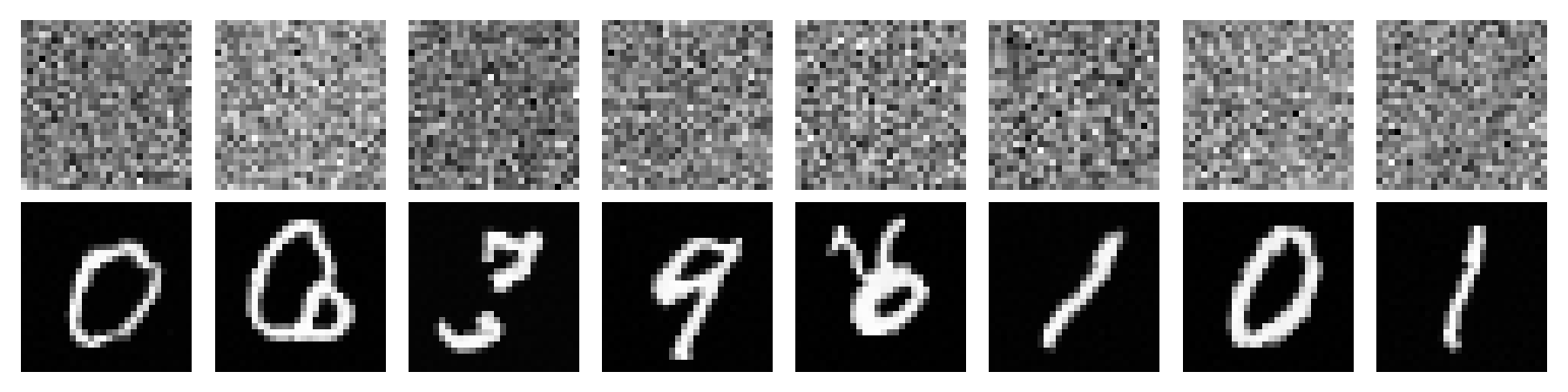
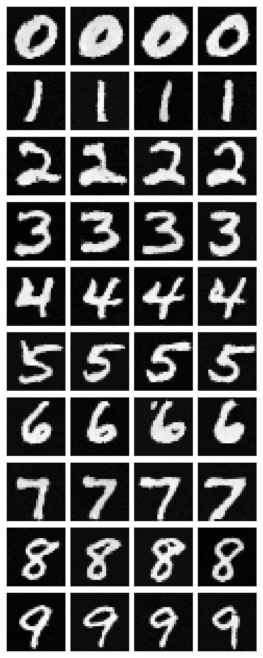
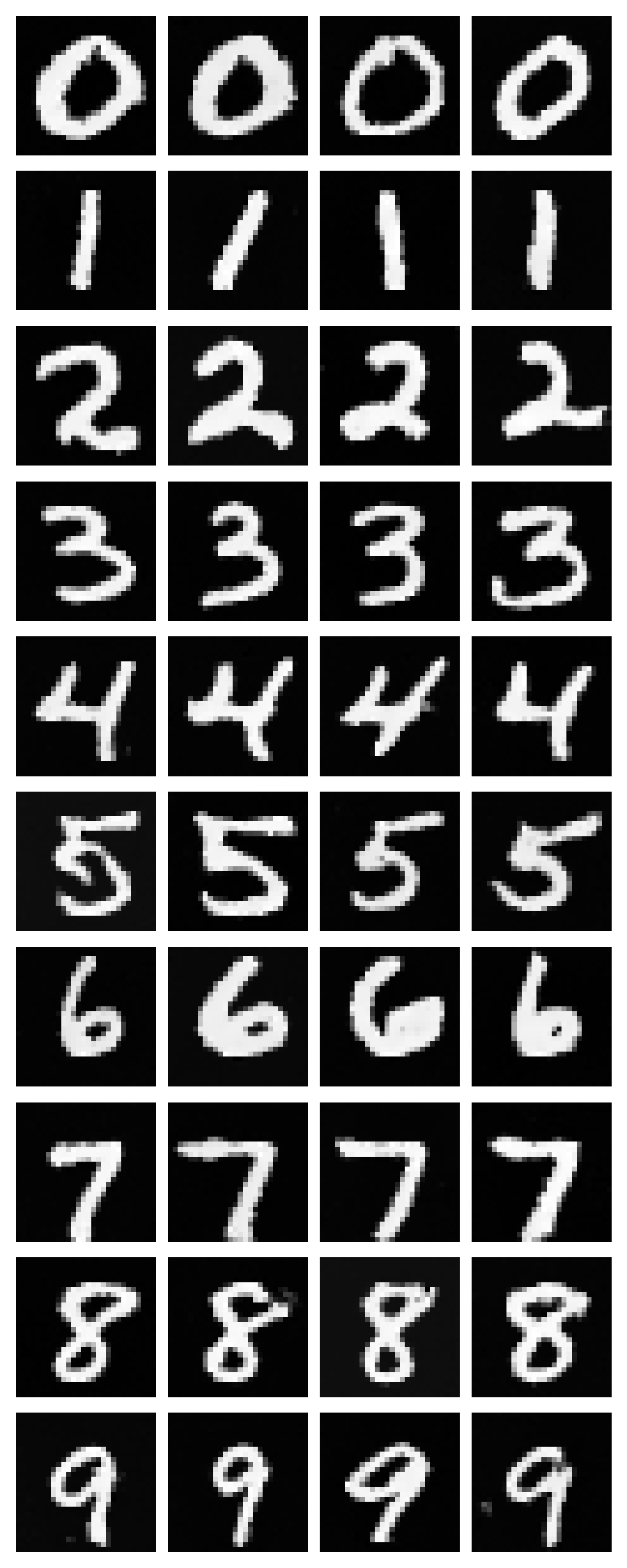
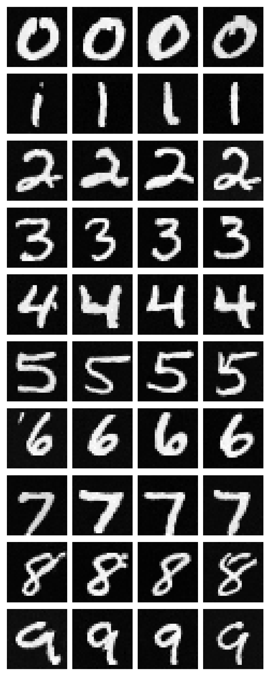
Sampling from class‑conditioned UNet
Class‑conditional sampling uses classifier‑free guidance to combine unconditional and conditional flows.
With CFG, the conditional signal is strengthened without changing the underlying sampler: \(\gamma\) trades off diversity and fidelity. The grids below show 4 samples per class; by later epochs the model typically produces more consistent digits per class and fewer cross‑class confusions.
I also tested removing the exponential learning‑rate scheduler and training with a fixed learning rate. This is generally possible, but there is a stability–speed tradeoff: a higher learning rate worked best for me (good but not perfect results), however it converged very quickly and then plateaued, with later epochs not improving much. Lowering the fixed learning rate makes updates safer, but can slow training and risks getting stuck, which is why I prefer using a scheduler.

No scheduler (fixed learning rate) – samples
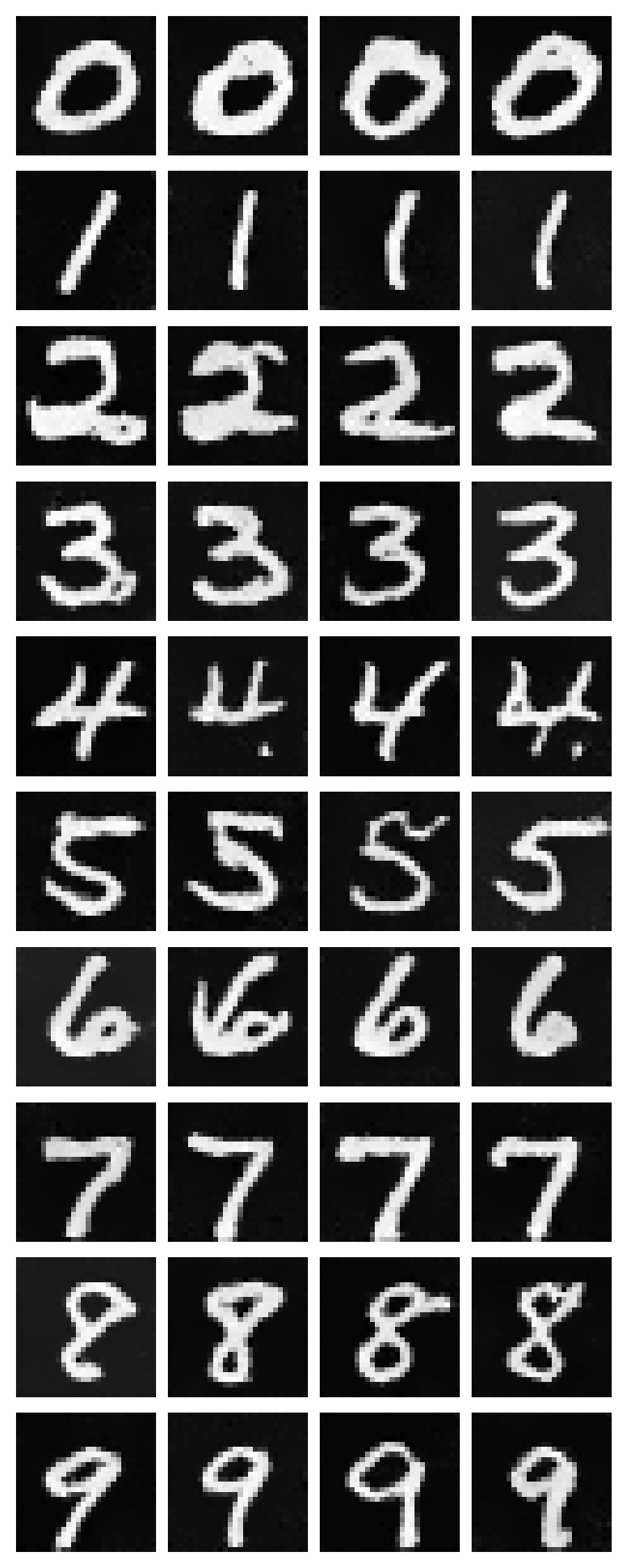
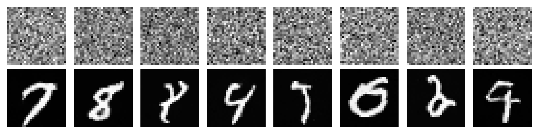
Bells & Whistles: improved time‑conditioned UNet
The time‑only model is improved by increasing the hidden dimension to 128 and extending training to 30 epochs, leading to sharper digits and fewer collapsed “average” shapes.
Increasing capacity (larger hidden dimension) helps the network represent a more accurate flow field, while longer training reduces underfitting. Qualitatively, later‑epoch samples show cleaner strokes and better separation between background and digit foreground compared to earlier epochs.